Many a times need arises for deriving insights from structured or unstructured data. To provide meaningful information from this large data, one incorporates data science to interpret data for decision-making.
Data Science is a field that comprises everything related to data cleansing, preparation and analysis. It is the method used to extract insights and information from data.
Gathr incorporates data science technique for deriving meaningful information from data. Using Gathr ML, PMML and H2O processors one can train models as well as score models for streaming and batch data.
Making predictions on real-time data streams or on a batch of data involves building an offline model and applying it to a stream. Models incorporate one or more machine-learning algorithm that is trained using the collected data.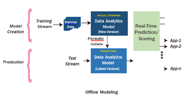
We support models that are created using ML, H2O, and PMML. In addition, we support some of the R models (created in PMML) to be used for scoring on data in Gathr.
ML Analytics processor enables you to use predictive models built on top of ML package.
ML provides higher-level API built on top of data frames that helps you to create and tune practical machine learning pipelines.
The documentation of ML Models is divided in the following section:
• Training
• Prediction (Model Scoring)
Models can be trained through Gathr with the help of ML processors. These models will be built on top of an ML package.
Model Training can only be performed on Batch Data.
You can connect multiple models of different or same algorithm and train model on the same message in a single pipeline.
Note: Intermediate columns calculated through transformations from one analytics processor will not be available on the next analytics processor if multiple analytics processor is trained in one pipeline.
You have eight algorithms under ML that supports Model Training and Scoring.
The data flow for all these models include a wizard-like flow, which is shown in the figure below:
Note: For the following models, Post-Processing, Model Evaluation and Hyper Parameters are not mandatory.
Isotonic Regression belongs to the family of Regression algorithms. It gives an approximate series of one-dimensional observations with a non-decreasing function. Isotonic Regression Analytics processor is used to analyze data using ML Isotonic Regression Model.
To use an Isotonic Regression Model in Data Pipeline, drag and drop the model component to the pipeline canvas and right click on it to configure.
The Configuration window of every ML model is same.
After Configuration tab comes, Feature Selection tab. (which is also same for all the models except K Means).
Once Feature Selection is done, perform Pre-Processing on the data before feeding it to the Model. The configuration settings are same for all the ML models.
Then configure the Model using Model Configuration. Following tabs are generated for this Model:
Field | Description |
|---|---|
Label Column | Column name which will be treated as label column while training a model. |
Feature Column | Column name which will be treated as feature column while training a model. |
Isotonic | Specifies whether Isotonic is True or False When selected True,isotonic regression is isotonic (monotonically increasing) When selected False, isotonic regression is antitonic (monotonically decreasing). |
After Model Configuration, Post-Processing is done, Model Evaluation can be performed.
Then, apply the Hyper Parameters on the model to enable tuning your configuration; after which you can simply add notes and save the Configuration.
Regression is an approach for modeling the relationship between a scalar dependent variable and one or more explanatory variables (or independent variables).
Regression Analytics processor is used to analyze data using ML LinearRegressionModel.
To use a Linear Regression Model in Data Pipeline, drag and drop the model component to the pipeline canvas and right click on it to configure.
The Configuration window of every ML model is same.
After Configuration tab comes, Feature Selection tab. (which is also same for all the models except K Means).
Once Feature Selection is done, perform Pre-Processing on the data before feeding it to the Model. The configuration settings are same for all the ML models.
Then configure the Model using Model Configuration. Following tabs are generated for this Model:
Field | Description |
|---|---|
Label Column | Column name which will be treated as label column while training a model. |
Feature Column | Column name which will be treated as feature column while training a model. |
Prediction Column | Select the columns to be predicted. |
Num Iterations | Number of iterations of gradient descent to run per update. |
ElasticNet Parameter | Sets the ElasticNet mixing parameter for the model. For alpha = 0, the penalty is an L2 penalty. For alpha = 1, it is an L1 penalty. For alpha (0, 1), the penalty is a combination of L1 and L2. Default is 0.0, which is an L2 penalty. |
Regularization Parameter | Regularization parameter for model training. |
After Model Configuration, Post-Processing is done, Model Evaluation can be performed.
Apply the Hyper Parameters on the model to enable tuning your configuration; after which you can simply add notes and save the Configuration.
Decision trees and their ensembles are popular methods for the machine learning tasks of classification and regression. Decision trees algorithms are easy to interpret, they handle categorical features, extend to the multi-class classification setting, do not require feature scaling, and are able to capture non-linearity and feature interactions.
Decision Tree Analytics processor is used to analyze data using ML’s DecisionTreeClassificationModel and DecisionTreeRegressionModel.
To use a Decision Tree Model in Data Pipeline, drag and drop the model component to the pipeline canvas and right click on it to configure:
The Configuration window of every ML model is same.
After Configuration tab comes, Feature Selection tab. (which is also same for all the models except K Means).
Once Feature Selection is done, perform Pre-Processing on the data before feeding it to the Model. The configuration settings are same for all the ML models.
Then configure the Model using Model Configuration. Following tabs are generated for this Model:
Field | Description |
|---|---|
Label Column | Column name that will be treated as label column while training a model. |
Probability Column | Column name that holds the value of probabilities of predicted output. |
Prediction Column | Select the columns to be predicted. |
Feature Column | Column name which will be treated as feature column while training a model. |
Max Bins | Number of bins used when discretizing continuous features. |
Max Depth | Maximum depth of the tree that needs to be trained. This should be chosen carefully as it acts as a stopping criteria for model training. |
Impurity | Parameter which decides the splitting criteria over each node. Available options are Gini Impurity and Entropy for classification and Variance for Regression problems. |
Minimum Information Gain | Specifies the splitting criteria over each node. Calculated on the basis of Impurity parameter. |
Seed | Number used to produce a random number sequence that makes the result of algorithm reproducible. Specify the value of seed parameter that will be used for model training. |
Thresholds | Threshold parameter for the class range. Number of thresholds should be equal to Number of Output Classes. Mention only in case of Classification problems. |
After Model Configuration, Post-Processing is done, Model Evaluation can be performed.
Apply the Hyper Parameters on the model to enable tuning your configuration; after which you can simply add notes and save the Configuration.
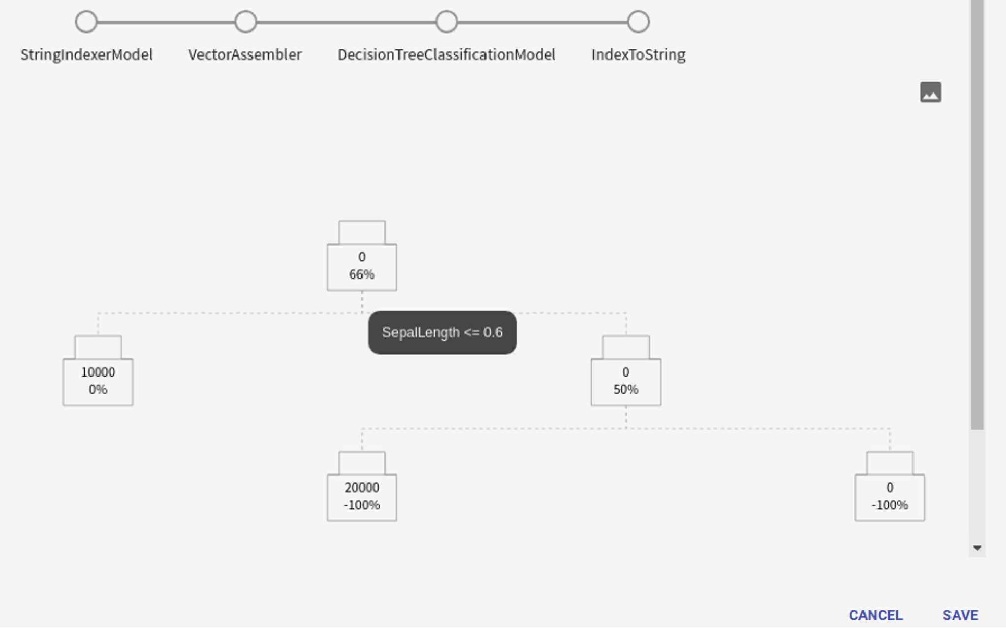
View Model
Decision Tree model support visualization of trained models. View Model feature is available in case of Prediction pipeline.
The trained tree model will be visualized as below:
Gradient-Boosted Trees (GBTs) are ensembles of decision trees. GBTs can be used for binary classification and for regression, using both continuous and categorical features.
Gradient-Boosted Trees Analytics processor is used to analyze data using ML’s GBTClassificationModel and GBTRegressionModel.
Note: GBTs does not support multi-label classification.
To use a GBT Model in Data Pipeline, drag and drop the model component to the pipeline canvas and right click on it to configure.
The Configuration window of every ML model is same.
After Configuration tab comes, Feature Selection tab. (which is also same for all the models except K Means).
Once Feature Selection is done, you will have to perform Pre-Processing on the data before feeding it to the Model. The configuration settings are same for all the ML models.
Then configure the Model using Model Configuration. Following tabs are generated for this Model:
Field | Description |
|---|---|
Label Column | Column name that will be treated as label column while training a model. |
Feature Column | Column name which will be treated as feature column while training a model. |
Probability Column | Column name that holds the value of probabilities of predicted output. |
Max Bins | Specify the value of max bins parameter for model training. |
Max Depth | Specify the maximum depth of the tree that needs to be trained. This should be chosen carefully as it acts as a stopping criteria for model training. |
Impurity | Parameter with the help of which split criteria is decided over each node. Available options are Gini Impurity and Entropy for classification problems and Variance for regression problems. |
Minimum Information Gain | Calculated on the basis of Impurity parameter. Specifies actually the splitting criteria over each node. Information gained using any feature column over a particular node should be more than this parameter value, so that tree can be split on the basis of that feature on that node. |
Seed | Specify seed parameter value. This value will be used for model training. |
Loss Type | Loss function which GBT tries to minimize. Supported options are “squared” (L2) and “absolute” (L1) for regression problems and logistic for classification problems. |
Max Iterations | Number of Iterations for building ensemble of trees. Number of Output trees is equal to the max iterations specified. This acts as one of the stopping criteria for model training. |
subSamplingRate | Specifies the size of the dataset used for training each tree in the forest, as a fraction of the size of the original dataset. The default (1.0) is recommended, but decreasing this fraction can speed up training. |
Step Size | Defines the learning rate. This determines the impact of each tree model on the outcome. GBT works by starting with an initial estimate that is updated using the output of each tree. The learning parameter controls the magnitude of this change in the estimates. Lower values are generally preferred as they make the model robust to the specific characteristics of tree and thus allowing it to generalize well. Lower values would require higher number of trees to model all the records and will be computationally expensive. |
After Model Configuration, Post-Processing is done, Model Evaluation can be performed.
Apply the Hyper Parameters on the model to enable tuning your configuration; after which you can simply add notes and save the Configuration.
Random forests are ensembles of decision trees. Random forests combine many decision trees to reduce the risk of over fitting. Random forests can be used for binary and multi-class classification and for regression, using both continuous and categorical features.
Random Forest Trees Analytics processor is used to analyze data using ML’s RandomForestClassificationModel and RandomForestRegressionModel.
To use a Random Forest Tress Regression Model in Data Pipeline, drag and drop the model component to the pipeline canvas and right click on it to configure.
The Configuration window of every ML model is same.
After Configuration tab comes, Feature Selection tab. (which is also same for all the models except K-Means).
Once Feature Selection is done, perform Pre-Processing on the data before feeding it to the Model. The configuration settings are same for all the ML models.
Then configure the Model using Model Configuration. Following tabs are generated for this Model:
Field | Description |
|---|---|
Label Column | Column name that will be treated as label column while training a model. |
Probability Column | Column name that holds the value of probabilities of predicted output. |
Feature Column | Column name which will be treated as feature column while training a model. |
Max Bins | Specify the value of max Bins parameter for model training. |
Max Depth | Specify the depth of the tree that needs to be trained. This should be chosen carefully as it acts as a stopping criteria for model training. |
Impurity | Parameter that decides the splitting criteria over each node. Available options are Gini Impurity and Entropy for classification and Variance for regression problems. |
Minimum Information Gain | Calculated based on Impurity parameter. Specifies actually the splitting criteria over each node. Information gained using any feature column over a particular node should be more than this parameter value, so that tree can be split based on that feature on that node. |
Seed | Number used to produce a random number sequence that makes the result of algorithm reproducible. Specify the value of seed parameter that will be used for model training. |
Thresholds | Specify the threshold parameter for class range. Number of thresholds should be equal to number of output classes. Required only in case of Classification problems |
Number of Trees | Number of trees in the forest. Increasing the number of trees will decrease the variance in predictions, improving the model’s test-time accuracy. Training time increases roughly linearly in the number of trees. |
Feature Subset Strategy | Number of features to use as candidates for splitting at each tree node. The number is specified as a fraction or function of the total number of features. Decreasing this number will speed up training, but can sometimes impact performance if too low. |
Sub Sampling Rate | Size of the dataset used for training each tree in the forest, as a fraction of the size of the original dataset. The default (1.0) is recommended, but decreasing this fraction can speed up training. |
After Model Configuration, Post-Processing is done, Model Evaluation can be performed.
Apply the Hyper Parameters on the model to enable tuning your configuration; after which you can simply add notes and save the Configuration.
Logistic regression is a popular method to predict a categorical response. A special case of generalized linear models predicts the probability of the outcomes. It can be used for both binary and multi-class classification problems.
Logistic Regression Analytics processor is used to analyze data using ML’s LogisticRegressionModel.
To us e a Logistic Regression Model in Data Pipeline, drag and drop the model component to the pipeline canvas and right-click on it to configure.
The Configuration window of every ML model is same.
After Configuration tab comes, Feature Selection tab. (which is also same for all the models except K-Means).
Once Feature Selection is done, perform Pre-Processing on the Model. The configuration settings are same for all the ML models.
Then configure the Model using Model Configuration. Following tabs are generated for this Model:
Field | Description |
|---|---|
Label Column | Column name that will be treated as Label column while training a model. |
Probability Column | Column name that holds the value of probabilities of predicted output. |
Feature Column | Column name which will be treated as feature column while training a model. |
Thresholds | Specify the threshold parameter for class range. Number of thresholds should be equal to Number of Output Classes. |
ElasticNet Param | Specify the value for ElasticNet Parameter for model training |
Regularization Parameter | Specify the value for Regularization Parameter for model training |
Max Iterations | Number of Iterations for building ensemble of trees. Number of Output trees is equal to the max iterations specified. This acts as one of the stopping criteria for model training. |
Fit Intercept | Whether to fit an intercept term or not. |
After Model Configuration, Post-Processing is done, Model Evaluation can be performed.
Apply the Hyper Parameters on the model to enable tuning your configuration; after which you can simply add notes and save the Configuration.
Naive Bayes are a family of simple probabilistic classifiers based on applying Bayes’ theorem with strong (naive) independence assumptions between the features. Currently, it supports both multinomial Naive Bayes and Bernoulli Naive Bayes.
Naive Bayes Analytics processor is used to analyze data using ML’s NaiveBayesModel.
To use a Naïve Bayes Model in Data Pipeline, drag and drop the model component to the pipeline canvas and right-click on it to configure.
The Configuration window of every ML model is same.
After Configuration tab comes, Feature Selection tab. (which is also same for all the models except K Means).
Once Feature Selection is done, perform Pre-Processing on the data before feeding it to the Model. The configuration settings are same for all the ML models.
Then configure the Model using Model Configuration. Following tabs are generated for this Model:
Field | Description |
|---|---|
Label Column | Column name which will be treated as label column while training a model. |
Probability Column | Column name which holds the probability value of the predicted output. |
Feature Column | Column name which will be treated as feature column while training a model. |
Model Type | Model Type for Naïve Bayes Classifier default is multinomial. Other model type supported is Bernoulli |
Thresholds | Specify the threshold parameter for class range. Number of thresholds should be equal to Number of Output Classes. |
Max Iterations | Number of Iterations for building ensemble of trees. Number of Output trees is equal to the max iterations specified. This acts as one of the stopping criteria for model training |
After Model Configuration, Post-Processing is done, Model Evaluation can be performed.
Apply the Hyper Parameters on the model to enable tuning your configuration; after which you can simply add notes and save the Configuration.
K-Means is one of the most commonly used clustering algorithms that clusters the data points into a predefined number of clusters. K-Means Analytics processor is used to analyze data using ML’s K-means Model.
To use a K-Means Model in Data Pipeline, drag and drop the model component to the pipeline and right click on it to configure.
The Configuration window of every ML model is same.
After Configuration tab comes, Feature Selection tab. (which is also same for all the models except K Means).
Once Feature Selection is done, perform Pre-Processing on the data before feeding it to the Model. The configuration settings are same for all the ML models.
Then configure the Model using Model Configuration. Following tabs are generated for this Model:
Field | Description |
|---|---|
Max Iterations | Number of Iterations for building ensemble of trees. Number of Output trees are equal to the max iterations specified. This acts as one of the stopping criteria for model training. |
Init Step | Parameter for the number of steps for the k-means|| initialization mode. This is an advance setting. Must be > 0. |
Feature Column | Column name which will be treated as feature column while training a model. |
Seed | Specify seed parameter value. This value will be used for model training. |
Tol | Set the convergence tolerance of iterations. Smaller value leads to higher accuracy with the cost of more iterations. |
Number of Clusters | Sets the number of clusters. Must be > 1. |
Init Mode | Parameter for the initialization algorithm. This can be either “random” to choose random points as initial cluster centers, or “k-means||” to use a parallel variant of k-means++. |
The configuration page is common for all the ML Models except Tree based, Naive Bayes and Logistic Regression models. For rest of the models, following are the properties with screenshot:
Note: Algorithm Type parameter is required in case of all the tree algorithms only i.e. Decision Trees, Gradient-Boosted Trees and Random Forests.
Field Description Operation Type of operation to be performed by Analytics processor: Training: Select the option training, if you want to train new models. Prediction: Select the option prediction, if you want to give predictions over existing model. Message Name The name for the message configuration which acts as a metadata for the actual data. Model Name Name of the model to be used in the data pipeline. Description Summary or a brief description of the model. Tags Tags to be associated with the model. Version Comments A note about the model version. Algorithm Type Specifies whether the current algorithm is used for solving a classification problem or regression. Select the required algorithm from the drop-down list. Classification Type Type of Classification- Binary or Multiclass. Save Model On Enables to save model on HDFS or Gathr database. When selected HDFS, specify HDFS connection and path. When selected Gathr database, model will be saved to database.
For using analytics processor in both training and prediction mode, you have to explicitly specify Input Labels and Variables such as Continuous, Categorical and Text.
Note:
• In case of Isotonic Regression, specify Input Label and Continuous Variable.
• In case of K-Means, Input Label is not required, since it is used for clustering issues
. Field Description Input Label Input Label signifies the incoming message field, which will be considered as a label field for model training. Features User can provide all the continuous, categorical and text variables within the features field. Drop Null Records All the null records within the selected columns will get dropped here.
In Pre-Processing, the data is transformed or consolidated so that the resulting mining process is more efficient, and the patterns found are easier to understand.
Once features are selected on Features selection tab, you can apply various transformations using Pre-Processing tab.
All ML models require feature column to be Vector Data type. For transforming raw input fields into type Vector, use Pre-Processing transformations.
Following are the descriptions of all the transformations/algorithms supported by Gathr over various analytics processor.
Binarizer thresholds numerical features to binary (0/1) features. Feature values greater than the threshold are binarized to 1.0; values equal to or less than the threshold are binarized to 0.0.
Enter values in the following parameters:
Field | Description |
|---|---|
Input Columns | Input column name over which Binarizer transformation is to be applied. Note: If you wish to apply algorithm on multiple columns, apply Vector Assembler transformation before the algorithm. |
Output Column | Name of the output column which will contain the transformed values after Binarizer transformation is applied. |
Threshold | Threshold value to be used for binarization. Features greater than the threshold, will be binarized to 1.0. The features equal to or less than the threshold, will be binarized to 0.0. Default: 0.0 |
Output Size Hint | Mention the size of the output Vector which will be generated after transformation is applied |
Output Size Handle Invalid | Parameter for handling invalid vectors. Invalid vectors include nulls and vectors with the wrong size. The options are “skip” (filter out rows with invalid vectors), “error” (throw an error) and “optimistic” (do not check the vector size, and keep all rows). Default is “error” |
Bucketizer transforms a column of continuous features to a column of feature buckets.
For configuration of Bucketizer Transformation, select algorithm Bucketizer.
Enter values in the following parameters:
Field | Description |
|---|---|
Input Columns | Input column name over which Bucketizer transformation is to be applied. Note: If you wish to apply algorithm on multiple columns, apply Vector Assembler transformation before the algorithm. |
Output Column | Name of the output column which will contain the transformed values after Binarizer transformation is applied. |
Splits | Splits are used to define buckets. With n+1 splits, there are n buckets. Splits should be strictly increasing. Use –inf for negative infinity and +inf for positive infinity. |
Handle Invalid | With this parameter, one can decide what to do with the invalid records. The three options available are Keep/Skip/Error. Keep will keep the invalid value and put it in any of the buckets, Skip will skip that particular record and Error will raise an exception if invalid record is inputted for transformation. |
The Imputer transformer completes missing values in a dataset, either using the mean or the median of the columns in which the missing values are located. Imputer doesn’t support categorical features. By default, all null values in the input columns are treated as missing, and so are also imputed. The input columns should be of decimal type.
Field Description Input Columns Input column name over which Imputer transformation is to be applied. You can select multiple Input Columns. Output Column Name of the output columns. In the output column missing values will be replaced by the surrogate value for the relevant column. Note: You can select multiple columns in Output Column too. However the Input Column and Output Column will be mapping the first input column with first output column and so on and so forth. Strategy The imputation strategy. Available options are "mean" and "median". If "mean" is selected, then all the occurrences of missing values will be replaced with using the mean value of the column. If "median" is selected, then all the missing values will be replaced using the approximate median value of the column. Default is mean Missing Value The placeholder for the missing values. All occurrences of missingValue will be imputed. Note that null values are always treated as missing.
CountVectorizer aim to help convert a collection of text documents to vectors of token counts.
Field Description Input Columns Name of the input column over which Bucketizer transformation is to be applied Output Column Name of the output columns. Each output column will contain CountVector for the respective input column. Vocabulary Size Max size of the vocabulary. CountVectorizer will build a vocabulary that only considers the top vocabSize terms ordered by term frequency across the corpus. Minimum Document Frequency Specifies the minimum number of different documents a term must appear to be included in the vocabulary. If this is an integer >= 1, this specifies the number of documents the term must appear in and if this is a double in [0,1), then this specifies the fraction of documents Minimum Term Frequency Filter to ignore rare words in a document. For each document, terms with frequency/count less than the given threshold are ignored. If this is an integer >=1, then this specifies a count (of times the term must appear in the document) and if this is a double in [0,1), then this specifies a fraction (out of the document's token count). Output Size Hint Mention the size of the output Vector which will be generated after transformation is applied Output Size Handle Invalid Parameter for handling invalid vectors. Invalid vectors include nulls and vectors with the wrong size. The options are “skip” (filter out rows with invalid vectors), “error” (throw an error) and “optimistic” (do not check the vector size, and keep all rows). Default is “error”
HashingTF is a transformer which takes sets of terms and converts those sets into fixed-length feature vectors.
Field Description Input Columns Name of the input column over which HashingTF transformation is to be applied Output Column Name of the output columns. Each output column will contain CountVector for the respective input column. Number of Features Should be > 0. (default = 2^18) Output Size Hint Mention the size of the output Vector which will be generated after transformation is applied Output Size Handle Invalid Parameter for handling invalid vectors. Invalid vectors include nulls and vectors with the wrong size. The options are “skip” (filter out rows with invalid vectors), “error” (throw an error) and “optimistic” (do not check the vector size, and keep all rows). Default is “error”
The IDFModel takes feature vectors (generally created from HashingTF or CountVectorizer) and scales each column. Intuitively, it down-weights columns which appear frequently in a corpus.
Field | Description |
|---|---|
Input Columns | Name of the input column over which idf transformation is to be applied. |
Output Column | Name of the output columns. Each output column will contain CountVector for the respective input column. |
Output Size Hint | Mention the size of the output Vector which will be generated after transformation is applied |
Output Size Handle Invalid | Parameter for handling invalid vectors. Invalid vectors include nulls and vectors with the wrong size. The options are “skip” (filter out rows with invalid vectors), “error” (throw an error) and “optimistic” (do not check the vector size, and keep all rows). Default is “error” |
MaxAbsScaler transforms a dataset of Vector rows, rescaling each feature to range [-1, 1] by dividing through the maximum absolute value in each feature. It does not shift/center the data, and thus does not destroy any sparsity.
MaxAbsScaler computes summary statistics on a data set and produces a MaxAbsScalerModel. The model can then transform each feature individually to range [-1, 1].
Field Description Input Columns Name of the input column over which IndexToString transformation is to be applied Output Column Name of the output columns. Each output column will contain CountVector for the respective input column. Output Size Hint Mention the size of the output Vector which will be generated after transformation is applied Output Size Handle Invalid Parameter for handling invalid vectors. Invalid vectors include nulls and vectors with the wrong size. The options are “skip” (filter out rows with invalid vectors), “error” (throw an error) and “optimistic” (do not check the vector size, and keep all rows). Default is “error”
MinMaxScaler transforms a dataset of Vector rows, rescaling each feature to a specific range (specified by parameter-min/max).
Field Description Input Columns Name of the input column over which MinMaxScaler transformation is to be applied Output Column Name of the output columns. Each output column will contain CountVector for the respective input column. Minimum Value Lower bound after transformation, shared by all features. Maximum Value Upper bound after transformation, shared by all features. Output Size Hint Mention the size of the output Vector which will be generated after transformation is applied Output Size Handle Invalid Parameter for handling invalid vectors. Invalid vectors include nulls and vectors with the wrong size. The options are “skip” (filter out rows with invalid vectors), “error” (throw an error) and “optimistic” (do not check the vector size, and keep all rows). Default is “error”
One-hot encoding maps a column of label indices to a column of binary vectors, with at most one single value. This encoding allows algorithms which expect continuous features, such as Logistic Regression, to use categorical features. Field Description Input Columns Input column name over which One-Hot Encoder transformation is to be applied. You can add multiple input columns. Output Column Name of the output columns. Each output column will contain one-hot-encoded vector for the respective input column. Note: You can select multiple columns in Output Column too. However the Input Column and Output Column will be mapping the first input column with first output column and so on and so forth. Drop Last Whether to drop the last category in the encoded vector. Default value is true Handle Invalid Parameter for handling invalid values encountered during the transformation. Available options are “keep” (invalid data presented as an extra categorical feature) or “error” (throw an error). Default is "error”. Output Size Hint Mention the size of the output Vector which will be generated after transformation is applied Output Size Handle Invalid Parameter for handling invalid vectors. Invalid vectors include nulls and vectors with the wrong size. The options are “skip” (filter out rows with invalid vectors), “error” (throw an error) and “optimistic” (do not check the vector size, and keep all rows). Default is “error”
NGram takes as input a sequence of strings (e.g. the output of a Tokenizer). The parameter n is used to determine the number of terms in each n-gram. The output will consist of a sequence of n-grams where each n-gram is represented by a space-delimited string of n consecutive words. If the input sequence contains fewer than n strings, no output is produced.
Field Description Input Columns Name of the input column over which NGram transformation is to be applied. Output Column Name of the output columns. Each output column will contain CountVector for the respective input column. N-Gram Param Minimum n-gram length, >= 1. Default value is 2.
Normalizer is a transformer that transforms a dataset of Vector rows, normalizing each Vector to have unit norm. It takes parameter p, which specifies the p-norm used for normalization. (p=2 by default.) This normalization can help standardize your input data and improve the behavior of learning algorithms. Field Description Input Columns Name of the input column over which Normalizer transformation is to be applied Output Column Name of the output columns. Each output column will contain CountVector for the respective input column. Norm Normalize a vector to have unit norm using the given p-norm. P-norm value is given by this norm Param Output Size Hint Mention the size of the output Vector which will be generated after transformation is applied Output Size Handle Invalid Parameter for handling invalid vectors. Invalid vectors include nulls and vectors with the wrong size. The options are “skip” (filter out rows with invalid vectors), “error” (throw an error) and “optimistic” (do not check the vector size, and keep all rows). Default is “error”
PCA is a statistical procedure that uses an orthogonal transformation to convert a set of observations of possibly correlated variables into a set of values of linearly uncorrelated variables called principal components. A PCA class trains a model to project vectors to a low-dimensional space using PCA.
Field Description Input Columns Name of the input column over which PCA transformation is to be applied. Output Column Name of the output columns. Each output column will contain CountVector for the respective input column. Number of Principal Components Number of principal components. Output Size Hint Mention the size of the output Vector which will be generated after transformation is applied. Output Size Handle Invalid Parameter for handling invalid vectors. Invalid vectors include nulls and vectors with the wrong size. The options are “skip” (filter out rows with invalid vectors), “error” (throw an error) and “optimistic” (do not check the vector size, and keep all rows). Default is “error”.
StandardScaler transforms a dataset of Vector rows, normalizing each feature to have unit standard deviation and or zero mean.
Field Description Input Columns Name of the input column over which StandardScaler transformation is to be applied. Output Column Name of the output columns. Each output column will contain CountVector for the respective input column. With Std Dev Whether to scale the data to unit standard deviation or not. With Mean Whether to center the data with mean before scaling or not. Output Size Hint Mention the size of the output Vector which will be generated after transformation is applied Output Size Handle Invalid Parameter for handling invalid vectors. Invalid vectors include nulls and vectors with the wrong size. The options are “skip” (filter out rows with invalid vectors), “error” (throw an error) and “optimistic” (do not check the vector size, and keep all rows). Default is “error”
Stop words are words which should be excluded from the input, characteristically because the words appear frequently and do not carry much meaning.
StopWordsRemover takes as input a sequence of strings (e.g. the output of a Tokenizer) and drops all the stop words from the input sequences. The list of StopWords is specified by the StopWords parameter.
Field Description Input Columns Name of the input column over which StandardScaler transformation is to be applied. Output Column Name of the output columns. Each output column will contain CountVector for the respective input column. Load Default Stop Words When you check this checkbox it asks for input language of which you want to pick default stop words to be removed by StopWordsTransformer. Some of the options include English, French, Spanish etc. Language English Case Sensitive Whether stop words are case sensitive or not
Tokenization is the process of taking text (such as a sentence) and breaking it into individual terms (usually words). A simple Tokenizer class provides this functionality.
Field Description Input Columns Name of the input column over which Tokenizer transformation is to be applied. Output Column Name of the output columns. Each output column will contain CountVector for the respective input column. Pattern Regex pattern used to match delimiters if [[gaps]] is true or tokens if [[gaps]] is false. Gaps Indicates whether regex splits on gaps (true) or matches tokens (false).
VectorAssembler is a transformer that combines a given list of columns into a single vector column.
Field Description Input Columns Input column name over which VectorAssembler transformation is to be applied Output Column Name of the output columns. Each output column will contain CountVector for the respective input column.
VectorIndexer helps index categorical features in datasets of Vectors. It can both automatically decide which features are categorical and convert original values to category indices.
For Configuration of VectorIndexer Transformation one has to select as algorithm VectorIndexer on the transformations tab. It asks for various configuration fields. Their description is as below:
Field Description Input Columns Name of the input column over which VectorIndexer transformation is to be applied. Output Column Name of the output columns. Each output column will contain CountVector for the respective input column. Max Categories Threshold for the number of values a categorical feature can take. If a feature is found to have > maxCategories values, then it is declared continuous. Must be >= 2. Output Size Hint Mention the size of the output Vector which will be generated after transformation is applied Output Size Handle Invalid Parameter for handling invalid vectors. Invalid vectors include nulls and vectors with the wrong size. The options are “skip” (filter out rows with invalid vectors), “error” (throw an error) and “optimistic” (do not check the vector size, and keep all rows). Default is “error”
Word2Vec maps each word to a unique fixed-size vector.
For configuration of Word2Vec Transformation, one has to select as algorithm Word2Vec on the transformations tab. It asks for various configuration fields. Their description is as below:
Field Description Input Columns Name of the input column over which Word2Vec transformation is to be applied. Output Column Name of the output columns. Each output column will contain CountVector for the respective input column. Vector Size The dimension of the code that you want to transform from words. Default value is 100. Window Size The window size (context words from [-window, window]) default 5 Step Size The step size. Min Count The minimum number of times a token must appear to be included in the word2vec model's vocabulary. Default value is 5. Max Iteration The max iteration. Max Sentence Length Set max sentence lengt.h Output Size Hint Mention the size of the output Vector which will be generated after transformation is applied. Output Size Handle Invalid Parameter for handling invalid vectors. Invalid vectors include nulls and vectors with the wrong size. The options are “skip” (filter out rows with invalid vectors), “error” (throw an error) and “optimistic” (do not check the vector size, and keep all rows). Default is “error”.
StringIndexer encodes a string column of labels to a column of label indices. The indices are in [0, numLabels), ordered by label frequencies, so the most frequent label gets index 0. The unseen labels will be put at index numLabels if user chooses to keep them. If the input column is numeric, we cast it to string and index the string values.
For configuration of StringIndexer Transformation, one has to select as algorithm StringIndexer on the transformations tab. It asks for various configuration fields. Their description is as below:
Field | Description |
|---|---|
Input Columns | Name of the input column over which StringIndexer transformation is to be applied |
Output Column | Name of the output columns. Each output column will contain CountVector for the respective input column. |
Handle Invalid | With this parameter, one can decide what to do with the invalid records. The three options available are Skip/Error. Skip will skip that particular record and Error will raise an exception if invalid record is inputted for transformation. |
Feature Hasher projects a set of categorical or numerical features into a feature vector of specified dimension. This is done using a hashing trick to map features to indices in the feature vector. Null (missing) values are ignored (implicitly zero in the resulting feature vector).
For configuration of Feature Hasher, one has to select the algorithm on the transformations tab. It asks for various configuration fields. The description is as below:
Field | Description |
|---|---|
Input Columns | Name of the input column over which Feature Hasher transformation is to be applied |
Output Column | Name of the output column which will contain the transformed feature vector. |
Num Features | Number of features. Should be greater than 0. (default = 2^18^) |
Categorical Columns | Numeric columns to treat as categorical features. By default only string and boolean columns are treated as categorical, so this param can be used to explicitly specify the numerical columns to treat as categorical. Note, the relevant columns must also be set in inputCols. |
Output Size Hint | Mention the size of the output Vector which will be generated after transformation is applied |
Output Size Handle Invalid | Parameter for handling invalid vectors. Invalid vectors include nulls and vectors with the wrong size. The options are “skip” (filter out rows with invalid vectors), “error” (throw an error) and “optimistic” (do not check the vector size, and keep all rows). Default is “error” |
Note: Model Training is not supported in streaming pipelines.
The post-processing tab enables you to perform transformations on model output before displaying the final result.
Currently, Gathr supports only one algorithm i.e IndexToString for post-processing.
IndexToString maps a column of label indices back to a column containing the original labels as strings. A common use case is to produce indices from labels with StringIndexer, train a model with those indices and retrieve the original labels from the column of predicted indices with IndexToString. However, you are free to supply your own labels.
Field | Description |
|---|---|
Input Columns | Name of the input column over which IndexToString transformation is to be applied |
Output Column | Name of the output columns. Each output column will contain CountVector for the respective input column. |
Labels | Labels to be used for transforming inputs indices into String. There are two options for doing this either user can reuse labels created in the pipeline earlier while any of the StringIndexer Transformations or it can specify new labels over here only. |
Select StringIndexer | Select the StringIndexer from the transformation chain on which IndexToString algorithm needs to be applied. |
Evaluate models on the metrics available for the ML algorithm.
Model Evaluation is configured using the following three properties:
Field | Description |
|---|---|
Enable Model Evaluation | Select the box for Enabling the model for evaluation. |
Train Ratio | Ratio in which incoming data will be split for training and testing. Value should be between 0 and 1. Example – 0.7 (70% data will be used for training and 30% for testing) |
Select Metric | The metric on which user wants to evaluate the model. |
Note: Elastic Search will be used in the background to store actual label of the data and model’s output to evaluate the model metrics.
Using this tab, you are able to optimize hyper parameters of algorithms used in the transformation chain.
Field | Description |
|---|---|
Execute Tuning | When selected, enables model tuning and evaluation. |
Validation Type | Tools used for tuning the model: Cross validation: In cross-validation, you make a fixed number of folds (or partitions) of the data, run the analysis on each fold, and then average the overall error estimate. Train Validation Split: Train Validation Split creates a single dataset pair. When Train Validation Split is selected, specify value for Train Validation Ratio. Note: If Enable Model Evaluation is checked under Model Evaluation tab, then Train Ratio parameter is not available, since you are already added train ratio in Model Evaluation Tab. |
Number of Folds | Specifies the number of folds for cross validation. Must be greater than or equal to two. Default value is three. |
Tuned Model Name | Name of the Model created after applying Hyper Parameter Training. |
Description | Summary or short description of the model. |
Tags | Tags to be associated with the model. |
Version Comments | A note about the model version. |
Metric for evaluation | Select the metric to be used for model evaluation. |
Train Ratio | Ratio between train and validation data. Must be between zero and 1. Default is 0.75 |
Tuned Model Name | Model created after Hyper Parameter model training. |
Connection Name | All HDFS connections will be listed here. Select the HDFS connection where model is to be saved. |
HDFS Path | Specify HDFS path for saving the model. |
Note: Connection Name and HDFS Path are populated when Select Click on the Add Notes tab. Enter the notes in the specified area.
Click on the SAVE button after entering all the information.
Once the model is trained using training pipelines, it is registered to be used for scoring in any pipeline.
To use a trained model in a pipeline for scoring, drag and drop the analytics processor and change the mode of analytics processor from training to prediction.
Field | Description |
|---|---|
Operation | Type of operation to be performed by Operator. It could be Training or Prediction operation. |
Algorithm Type | Select the Model Class, it could be Regression or Classification. |
Model Name | Name of the model to be created when the training model is activated or the model name to be used for the prediction when the prediction mode is activated. |
Message Name | Name of the message that will be used in the pipeline. |
Detect Anomalies | Select to detect anomalies in the input data. |
Anomaly Threshold | This is the threshold distance between a data point and a centroid. If any input data point’s distance to its nearest centroid exceeds this value then that data point will be considered as an anomaly. |
Is Anomaly Variable | Input message field that will contain the result of anomaly test i.e. it will be true if a data record is an anomaly or false otherwise. |
Note:
Operations, Message Name Model Name- Common for models
Anomaly options are only available for K means and Algorithm Type is available for Decision Tree, GBT ands Random Forest models.
Save the analytics processor and connect an emitter, for verifying the output.
Once the pipeline is saved, run it for predicting the output.
Using Externally Trained Models
For using externally trained model into Gathr, register the model from Register Entities tab.
For registering a model,
1.Click on the register entities section on the left pane.
2.After clicking on register, entities section move to register models tab.
3.Click on the (+) icon shown in the top-right corner of register models tab. A new window will open, enter model related parameters such as name of the model, whether pipeline model or not, API used for creating model and the algorithm type of the model. In case of Tree Ensemble based models, select, if the model is for classification problem or regression one.
4.After configuring the above fields, upload model for registration or provide HDFS path wherein the model is saved.
5.Validate the model by clicking validate model button, if it fails then the trained model is incorrect and if it is valid, register the model for prediction by clicking on the register model button.
6.Once the model is registered, you can use it for Prediction.
Note: You can only register models trained using ML and H20 API.
PMML stands for “Predictive Model Markup Language”. It is the de facto standard to represent predictive solutions. A PMML file may contain a myriad of data transformations (pre and post-processing) as well as one or more predictive models.
Its structure follows a set of pre-defined elements and attributes which reflect the inner structure of a predictive workflow: data manipulations followed by one or more predictive models.
Below mentioned is the list of PMML Models available in Gathr.
Logistic Regression is a classification algorithm. It is used to describe data and to explain the relationship between one dependent binary variable and one or more independent variables. It is used to predict a binary outcome like 1 or 0, yes or no, true or false given a set of independent variables.
Logistic Regression analytics processor will be used to perform prediction on the incoming data by using a PMML.
An existing PMML file can uploaded to the processor or a PMML can by created using the processor.
Configuring Logistic Regression Model
To add Logistic Regression model into your pipeline, drag Logistic Regression model to the canvas and right click on it to configure.
The Configuration Settings of Logistic Regression model are as follows:
Field | Description |
|---|---|
Schema | Select the message on which Logistics Regression is to be applied. |
Import PMML | Enables to import PMML file. Yes: when the Model is Imported, four tabs are enabled – Import and Download, which are to be followed in sequence. Also the model is validated and a success message is displayed or if the model is invalid a failure message will be displayed. No: If the Model is not imported and created, Download the Model option is enabled. |
Import | Import a PMML file. |
Validate Model | Checks the validity of the model. Validating a model is mandatory before viewing or testing the model. |
DOWNLOAD | Download the PMML Model that was created or imported. |
Add Configuration | Configure additional parameters in Key – Value pair. |
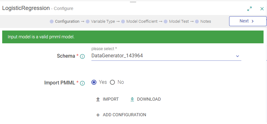
Logistic Regression can be processed in two ways:
Choose Import Model as Yes and click the Import button to load the PMML file.
Once the model is imported, following checks will be performed on the Model:
• The imported file must be a valid PMML file and it must have Logistic Regression model.
• The features and output defined in the model must be present in the selected message with the data type expected by model.
If the check fails, then the model will not be loaded in the processor and save features will be disabled. If above checks are met, then model can be saved.
Note:
• If the PMML model imported is not as per the analytics processor chosen, then validation of the model will throw an error.
a) All the values on screen will be read-only since an imported model cannot be edited.
b) If model variables are not defined in the message, they appear in red. This is to highlight that these fields need to be defined in the message, to consume the model in Gathr, as shown below: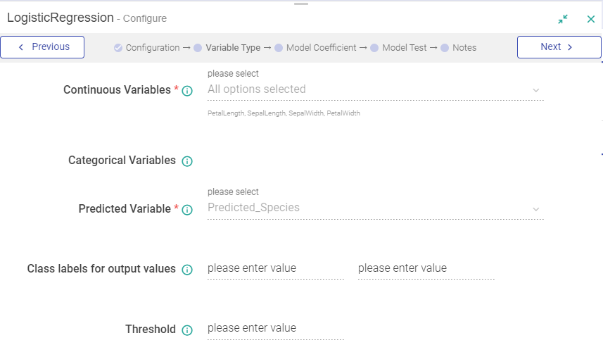
Since PMML model is imported, the Variables cannot be edited.
Note: If there is any Variable Type that is not defined in the message, the variables will appear in red.
If you want to classify the model output i.e. probability, then specify the threshold parameter, Low and High Classifiers under Variable Type. Threshold parameter takes a numeric value. The output value of the model is compared with the threshold, if the output is greater than threshold then the High classifier appear as output otherwise the Low classifier will appear.
After viewing the Variable Type, Click Next and Model Coefficients Page will open.
Click on Load Defined Variables to load the Variables and provide values against variables.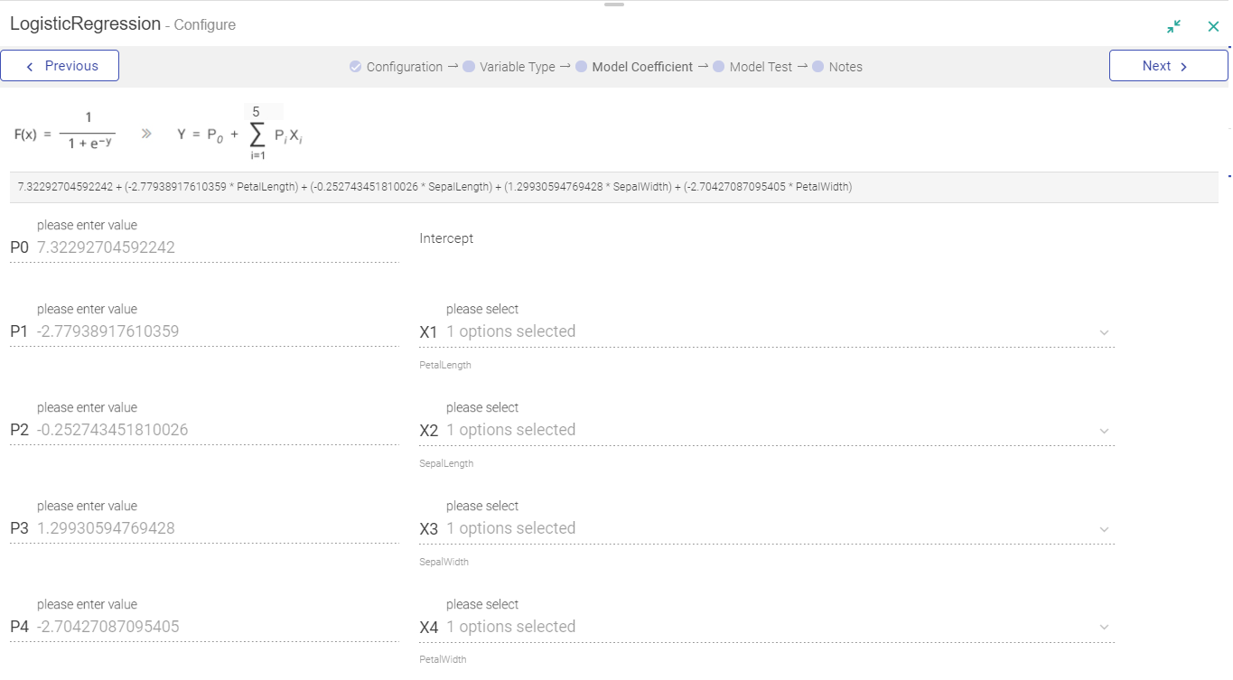
Now you can Test your Model with Values.
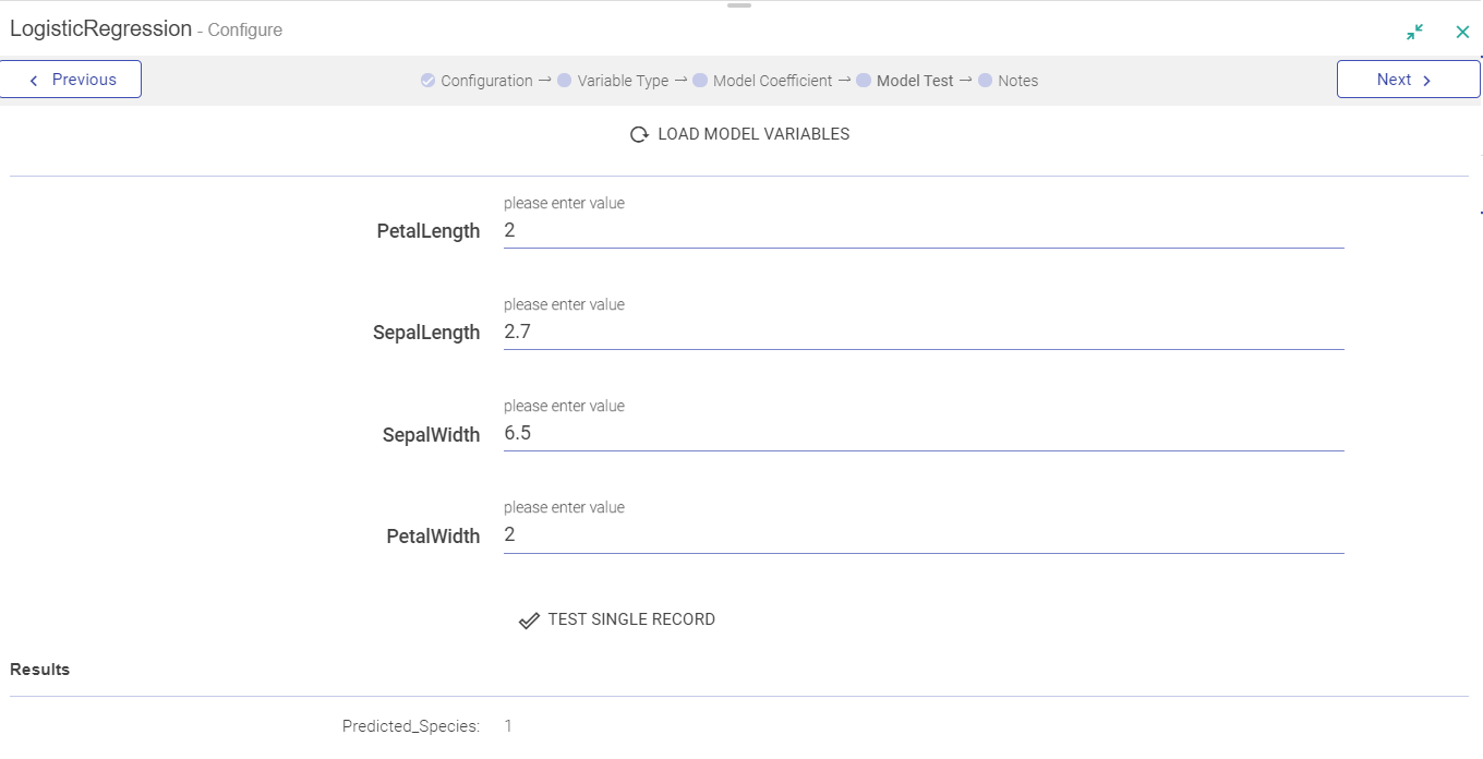
Once you have tested the mode, provide your notes in the add notes section and save the configuration.
Other option is to create your own PMML model.
If you want to create a PMML Logistic Regression model, follow the steps mentioned below:
Select a message from Message and select Import PMML as No.

Select Next, it will take you to Variable Type tab.

Select the Input Variables, which is Continuous and Categorical Variables.
Provide a name to the Predicted Variable (Output) and provide Class labels for output values and a Threshold value.
Click Next to view the Model Coefficients. All the model features defined on Variables Type screen can be used in Model Coefficients.
The screenshot above represents the generic formula for Logistic Regression, where P0 represents model Intercept and PiXi represents combination of Model Coefficient and Model feature respectively.
You can load all defined model features using Load Defined Variables link or choose one at a time from the list. You can specify the respective coefficients of the feature under coefficients column (PO-P8). If you are aware of the number of model variables to be used in model, specify the number in formula (above Sigma symbol) and those many rows will be automatically loaded on screen. In each row, you must specify the coefficient next to Pi and respective feature next to Xi, where i is the row number. Apart from features, a combination of continuous model features i.e. Interaction terms can also be defined as Xi.

Provide values to Probability and proceed to testing the Model.
Test the Model
Once the model is loaded, you can test the model with Model Test tab. Click Load Model to load and view the model.

Specify value of all model features and perform a single record test. The system will evaluate the model for this input and will show all the output parameters on screen.
Add Notes and save the Configuration.
Regression analytics processor is used to analyze data through Regression model. Regression analysis is used for estimating the relationship among variables. It helps to identify how the value of dependent variable changes when any one of the independent variable is changed, while other independent variables are fixed. It is used for prediction and forecasting.
To add Regression model into your pipeline, drag Regression model to the canvas and right click on it to configure.
The configuration settings of Regression model are as follows:
Field | Description |
|---|---|
Schema | Select the message on which Regression algorithm is to be applied. |
Import PMML | Enables to import PMML file. Yes: When the Model is Imported, four tabs are enabled – Import, Validate Model, View Model and Download, which are to be followed in sequence. No: If the Model is not imported and created, download the Model option is enabled. |
Validate Model | Checks the validity of the model. Validating a model is mandatory before Viewing or Testing the model. |
Download | Download the PMML Model that was created or imported |
Add Configuration | Configure additional parameters in Key – Value pair |
Regression can be processed in two ways:
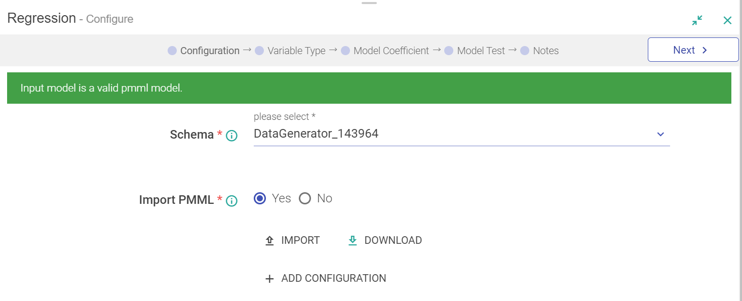
Choose Import Model as Yes and click the Import button to load the PMML file.
Once the model is imported, a message will be displayed validating if the model is valid or not.
Following checks will be performed:
• The imported file must be a valid PMML file and it must have Regression model. If this check fails, then the model will not be loaded in the processor, View Model and Save features are also disabled.
• The features and output defined in the model must be present in the selected message with the data type expected by model. If the message does not have certain attributes defined in model, then the View Model feature will be enabled but the model still cannot be saved. The error message in this case will explain which fields need to be defined.
When you click on next, Variable Type Tab opens the Variables as shown below:
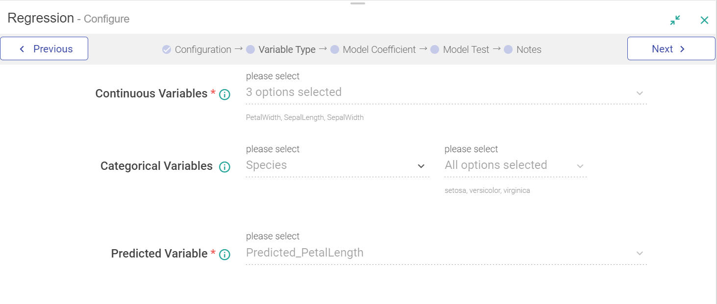
Since PMML model is imported, the Variables cannot be edited.
Note: If there is any Variable Type that is not defined in the message, the variables will appear in red.
After viewing the Variable Type, click Next and Model Coefficients page will open.
Click on Load Defined Variables to load the variables and provide values against variable
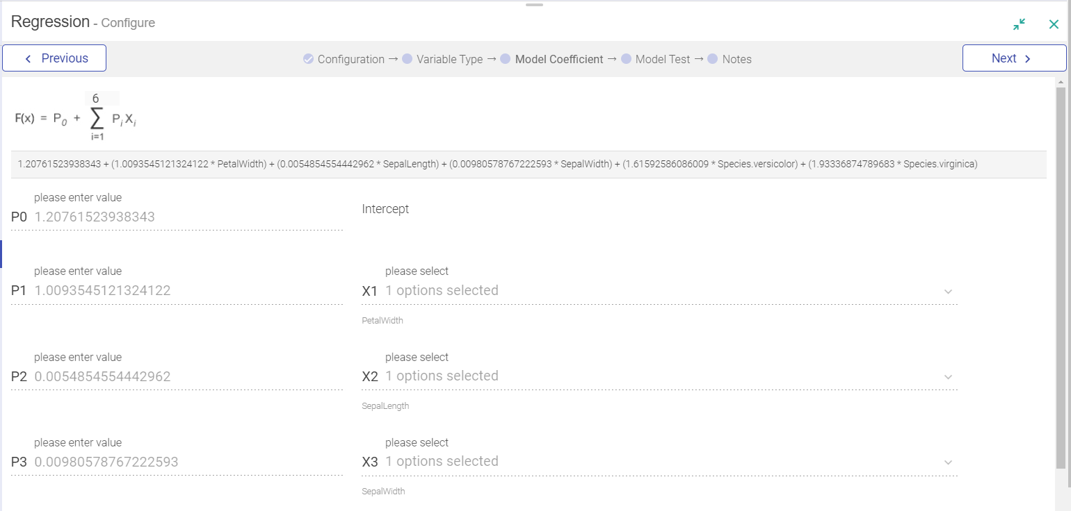
Now, test your Model with Values.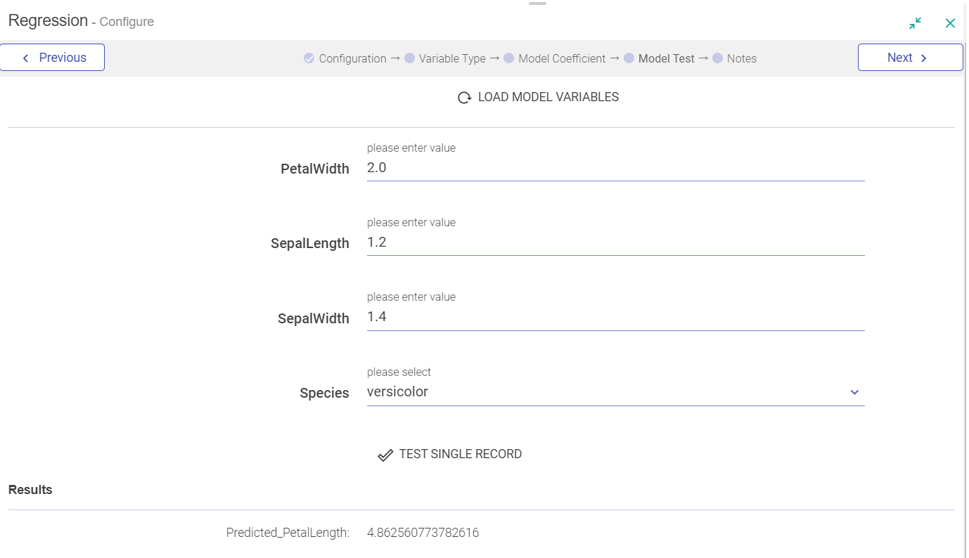
After the Model is tested, provide your notes in the Add Notes section and save the configuration.
Other option is to create your own PMML model.
If you want to create a PMML Regression model, choose Import PMML as No.
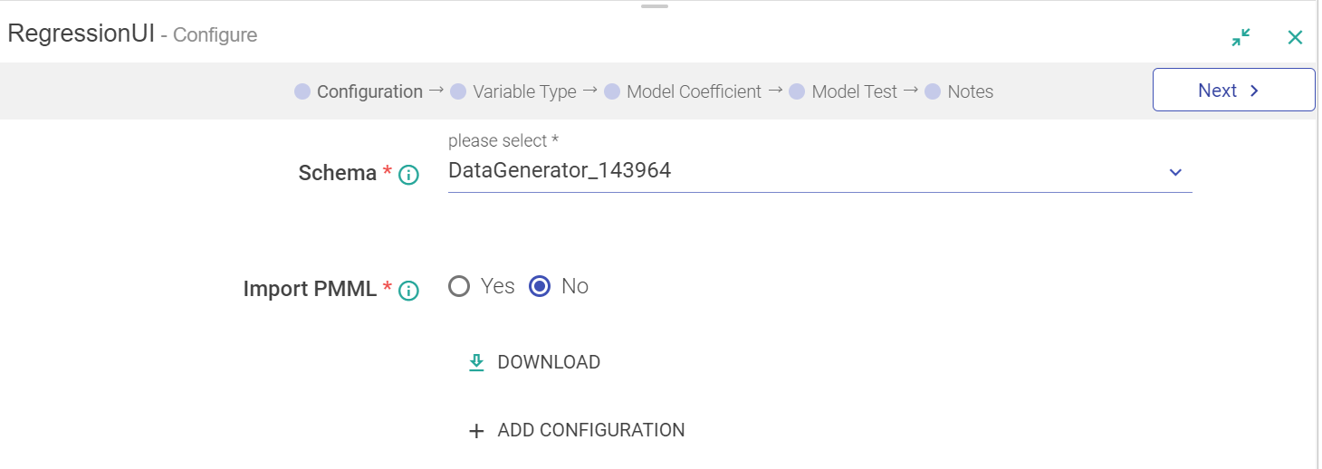
Variable Type
Variable Type and Model Coefficients tabs are enabled.
You must select the message field this variable corresponds to, along with the possible categories.
You can also use upload CSV option to populate categories for categorical variables under Categorical Variables via Add Variables, as shown below:
Model Coefficients
All the model features defined on Variable Type can be used on Model Coefficients page. The screenshot below represents the generic formula for Regression.
When you click on Next, you can test your model with values.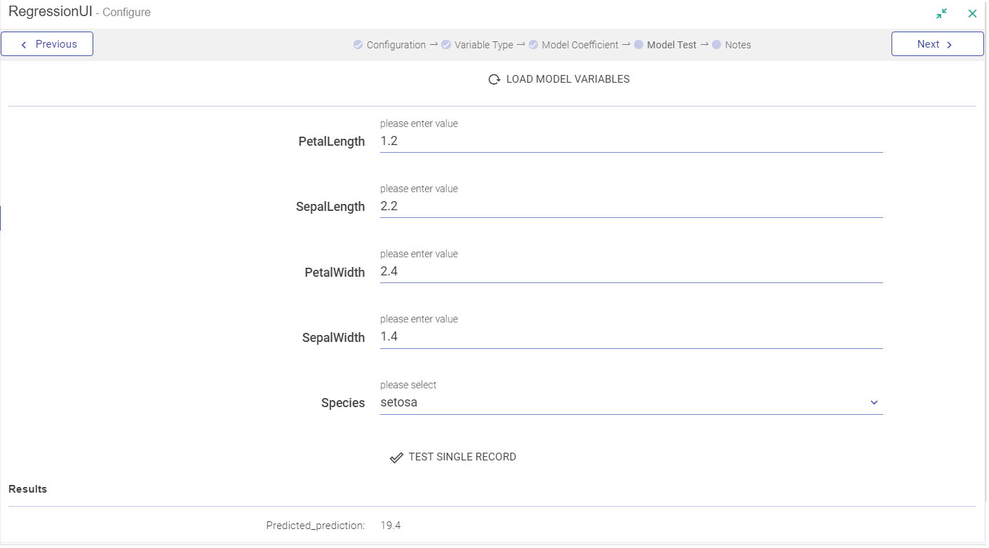
Once you have tested the mode, provide your notes in the Add Notes section and save the configuration.
Cluster Model Analytics processor is used to analyze data through Cluster model. It is commonly known as data clustering.
Data clustering is the task of diving a dataset into subset of similar items. Applying data clustering to a dataset generates group of similar data items. These groups are called clusters i.e. collection of similar data items.
Data clustering can help you identify, learn or predict the nature of new data items especially how new data can be linked for making predictions.
For example, in pattern recognition, analyzing pattern in the data like buying pattern in particular region or age group can assist you develop predictive analysis.
To add ClusterModel into your pipeline, drag ClusterModel to the canvas and right click on it to configure.
Field | Description |
|---|---|
Message | Select the message on which ClusterModel algorithm has to be applied. |
Import PMML | Enables to import PMML file. Yes: when the Model is Imported, four tabs are enabled – Import, Validate Model, View Model and Download, which are to be followed in sequence. No: If the Model is not imported and created, Download the Model option is enabled. |
Clustering | Clustering allows you to define various model features i.e. continuous variables, along with output variables, distance measure parameter and clustering parameters such as weight, cluster. |
Validate Model | Checks the validity of the model. Validating a model is mandatory before Viewing or Testing the model. |
Download | Downloads PMML file created either using Gathr UI or Import option. |
Add Configuration | Configure additional parameters in Key – Value pair. |
ClusterModel can be processed in two ways:
Choose import model as Yes and click the Import button to load the PMML file.
Once the model is imported, click on Validate Model.
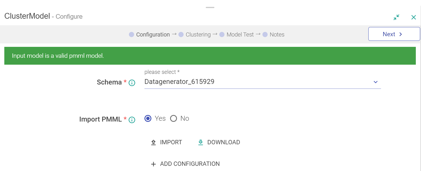
Checks will be performed on the model and if the defined variables does not match with the model then you will receive an error.
Create your own model through Gathr UI
If you have a ClusterModel definition and wish to create the model in Gathr. Choose import model as No and then clustering tab will be enabled.
You can add new cluster by clicking on add cluster link (plus icon)
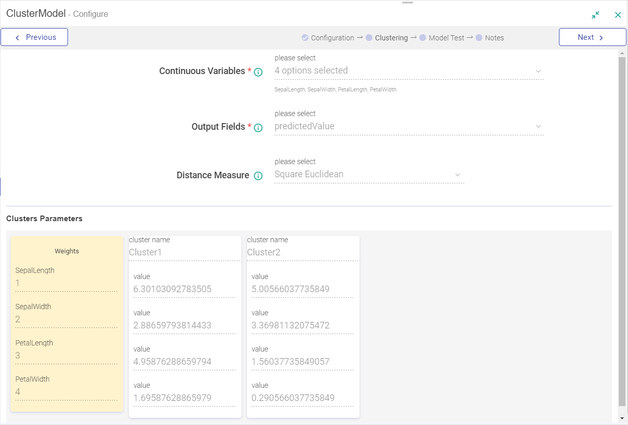
Test the model
Once the model is loaded (through UI or import) then you can test the model from Model Test screen. Click Load Model to load and view the Model.
Specify value to all model features and perform a single record test through Test Single Record. The system will evaluate the model for this input and will show all the output parameters on screen.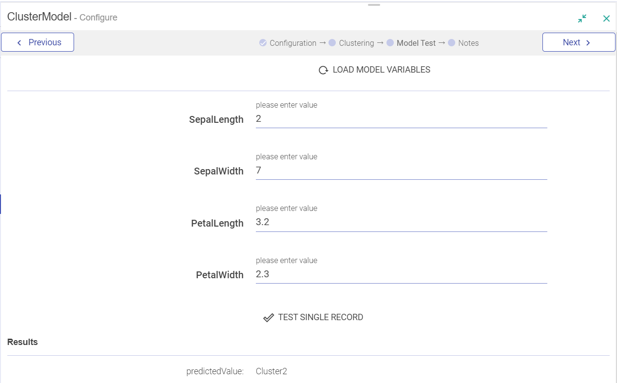
SupportVectorMachine analytics processor is used to analyze data through SupportVectorMachine model. SupportVectorMachine is a machine-learning algorithm that can be used for both classification and regression challenges. However, it is mostly used in classification problems.
Configuring SupportVectorMachine Model
To add SupportVectorMachine model into your pipeline, drag SupportVectorMachine model to the canvas and right click on it to configure.
Field | Description |
|---|---|
Schema | Select the message on which SupportVectorMachine algorithm has to be applied. |
Import PMML | Enables to import PMML file. Yes: when the Model is Imported, following tabs are enabled – Import and Download. |
Add Configuration | Configure additional parameters in Key – Value pair. |
Validate Model | Checks the validity of the model. Validating a model is mandatory before Viewing or Testing the model. |
SVM Processor can be processed in the following way:
If you have a PMML file representing SupportVectorMachine then import it. Click on Import button to load the file.
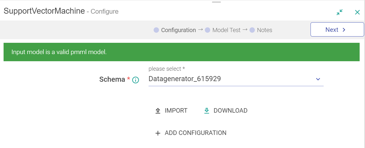
Once the model is imported, model validation with variable checks will be performed.
The next tab that is enabled is Test Model.
Test Model
You can test the model by clicking on Model Test Tab. Click Load Model to load and view the Model.
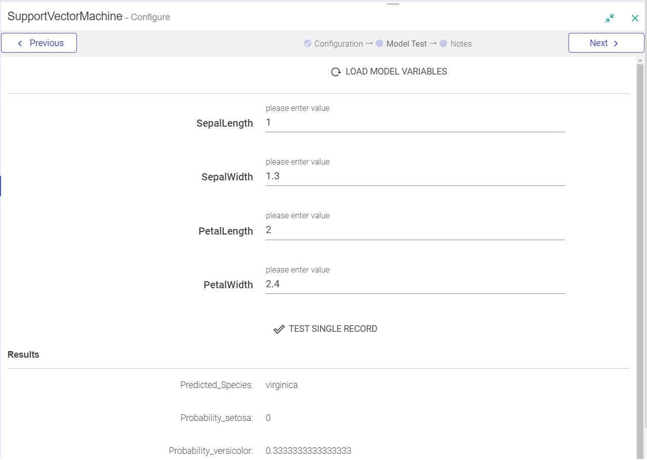
Specify value to all model features and perform a single record test through Test Single Record. The system will evaluate the model for this input and will show all the output parameters on screen.
NaiveBayes analytics processor is used to analyze data through NaïveBayes model. NaiveBayes model is easy to build and particularly useful for large data sets.
NaiveBayes classifier assumes that the presence of a particular feature in a class is unrelated to the presence of any other feature.
For example, a fruit may be considered an apple if it is red, round, and about 4 inches in diameter. Even if these features are dependent on each other or upon the existence of the other features, all of these attributes individually, contribute to the probability that this fruit is an apple and that is why it is known as ‘Naive’.
A Naive Bayesian model is simple to build, with no complex iterative parameter estimation that makes it specifically useful for very large datasets.
Field | Description |
|---|---|
Message | Select the message from the drop-down list on which analytics algorithm has to be applied. |
Import | Enables to import the PMML file |
Validate Model | Checks the validity of imported PMML file. |
Download | Downloads PMML file created either using Gathr UI or Import option. |
Add Configuration | Configure additional parameters in Key-Value pair. |
Input to this processor can only be provided as:
1. If you have a PMML file representing NaiveBayes, then you can directly import it. To do so click on Import button to load the file.
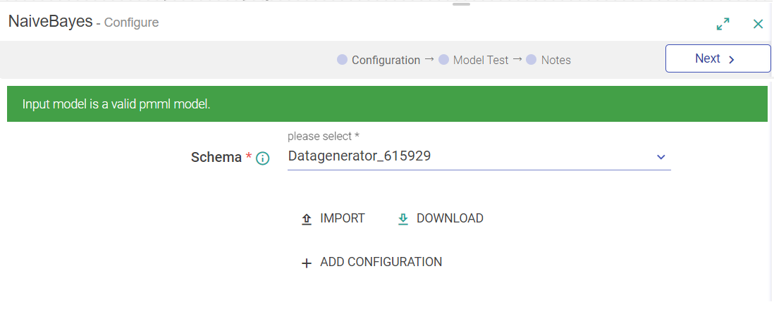
Once the model is imported, it should be validated. Following checks will be performed:
a) The imported file must be a valid PMML file and it must have NaiveBayes model. If this check fails, then the model will not be loaded in the processor and Save feature will be disabled.
b) The features and output defined in the model must be present in the selected message with the data type expected by model.
If the message does not have certain attributes defined in model then model cannot be saved, since without these features in message you will not able to execute the processor. The error message in this case will explain which fields needs to be defined.
Save the model once, the checks are met.
2. You can Download PMML file that you have imported.
3. Once the model is loaded, test the model using Model Test tab.
Test Model
Click on the Model Test tab. Click on Load Model button for loading the model fields.
Specify value for all the model features and perform a single record test by clicking on TEST SINGLE RECORD button. The system will evaluate the model for this input and will show all the output parameters on screen.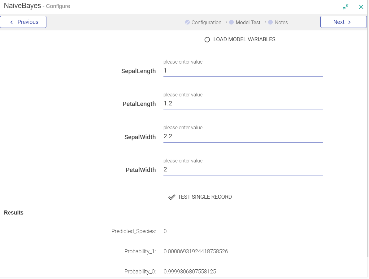
Add notes and save the configuration.
This analytics processor is used to analyze data through Ensemble model. Ensemble modeling is the process of running two or more related but different analytical models and then combining the results into a single score, which helps in improving the accuracy of predictive analytics and data mining applications.
Ensemble modeling offers one of the most convincing way to build highly accurate predictive models. Ensemble model combines multiple models together and delivers superior prediction power.
To add Ensemble model into your pipeline, drag Ensemble model to the canvas and right click on it to configure.
Field | Description |
|---|---|
Message | Select the message from the drop-down list on which analytics algorithm has to be applied. |
Import | Enables to import the PMML file |
Validate Model | Checks the validity of imported PMML file. |
Download | Downloads PMML file created either using Gathr UI or Import option. |
Add Configuration | Configure additional parameters in Key – Value pair. |
Input to this processor can only be provided as:
If you have a PMML file representing Ensemble, then you can import it. Click on Import button to load the file.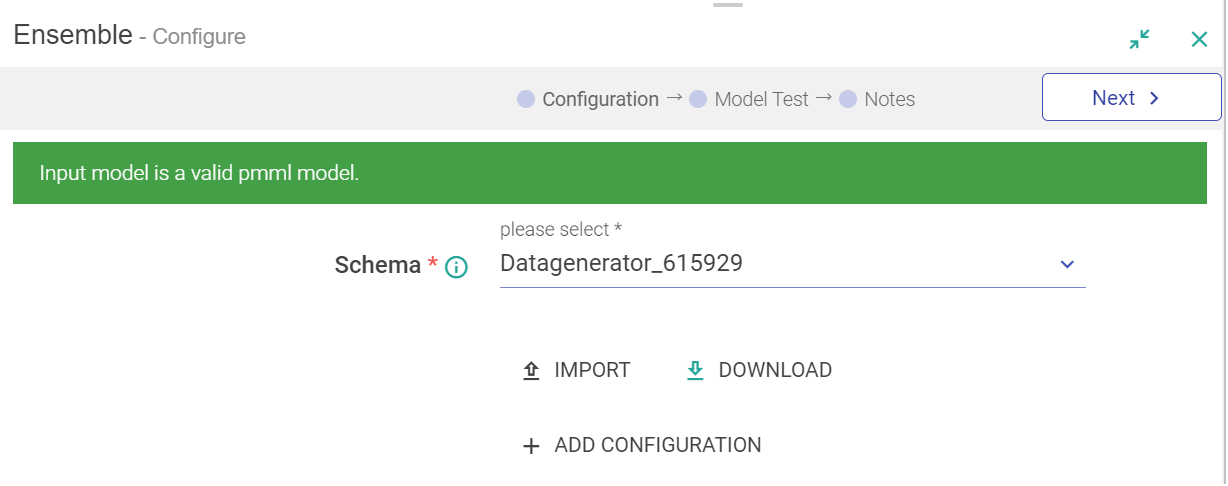
Once the model is imported, it is validated. Following checks will be performed:
The imported file must be a valid PMML file and it must have Ensemble model. If this check fails, then the model will not be loaded in the processor and Save features will be disabled.
The features and output defined in the model must be present in the selected message with the data type expected by model. In case the message does not have certain attributes defined in model, the error message will explain you, which fields needs to be defined.
If above checks are met, then model can be saved for execution.
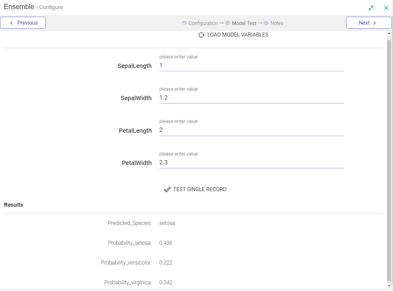
Once the model is loaded, you can test the model by clicking on Model Test tab.
If you click Load Model link, model features will appear on screen.
Add notes and save the configuration.
This analytics processor is used to analyze data through Neural Network model. A neural network is a powerful computational data model that is able to capture, represent complex input and output relationships.
Neural Networks are widely used for data classification, process past and current data to estimate future values.
Configuring Neural Network Model
To add Neural Network model into your pipeline, drag Neural Network model to the canvas and right click on it to configure.
Field | Description |
|---|---|
Schema | Select the message from the drop-down list on which Analytics algorithm has to be applied. |
Import | Enables to import PMML file. When the Model is Imported, two tabs are enabled – Import and Download. |
Download | Downloads PMML file created either using Gathr UI or Import option. |
Add Configuration | Configure additional parameters in Key–Value pair. |
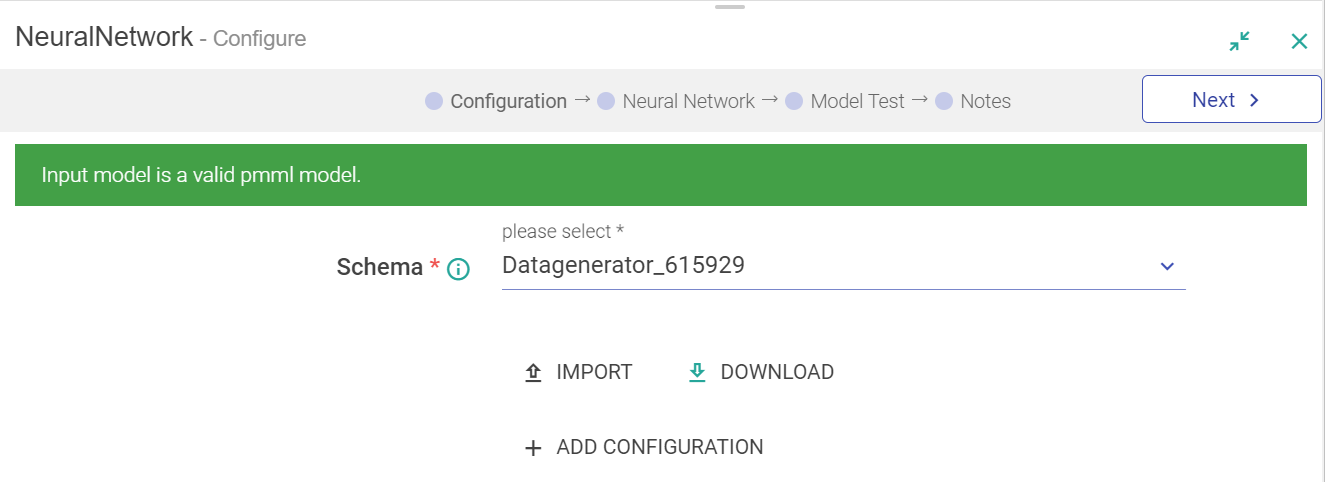
Input to this processor can only be provided as:
• If you have a PMML file, representing Neural Network then you can directly import it. Click the Import button to load the file.
Once the model is imported, it shall be validated.
Once it is validated, you can click on View Model. 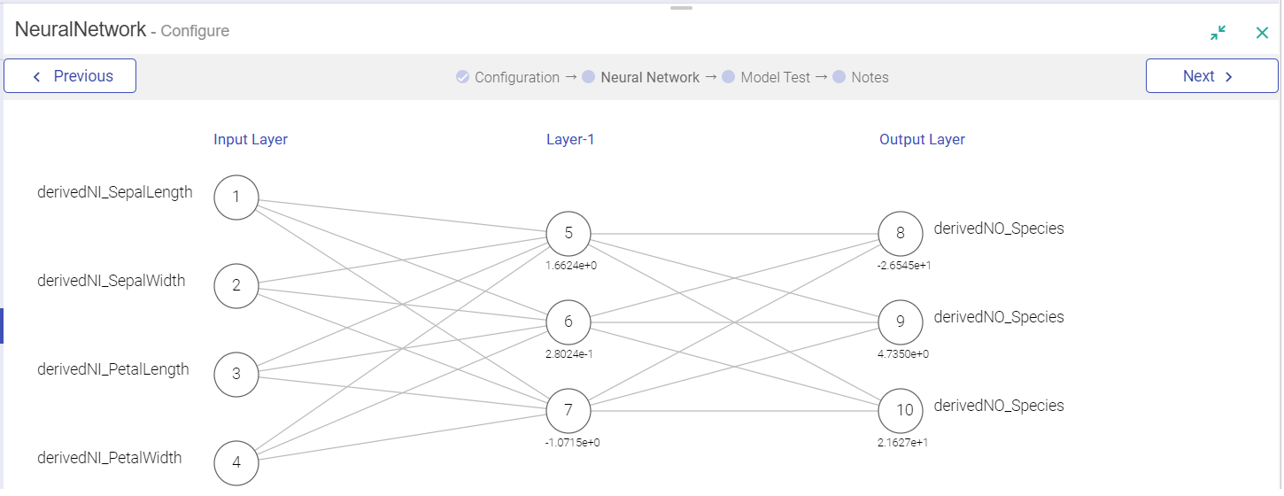
The Neural Network tab shows the graphical representation of the model. If you click on any weight or edge, you will be able to view the corresponding data.
We are able to visualize the Neutral Network. Weight specific to every edge is highlighted when you click on it.
Test Model
You can test the model by clicking on Model Test Tab. Click on Load Model button for loading the model fields. 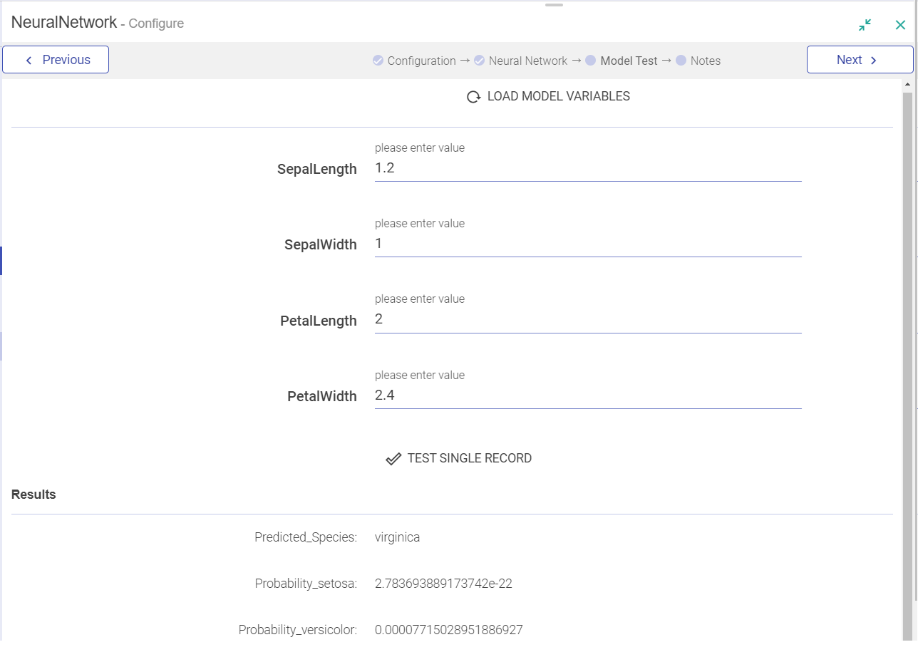
Specify value for all the model features and perform a single record test by clicking on TEST SINGLE RECORD button. The system will evaluate the model for this input and will show all the output parameters on screen.
This analytics processor is used to analyze data through Tree model. Tree based learning algorithms are considered to be one of the best learning methods.
This model provides high accuracy, stability and ease of interpretation. They are adaptable at solving either classification or regression problems.
Configuring Tree Model
To add Tree Model into your pipeline, drag Tree Model to the canvas and right click on it to configure.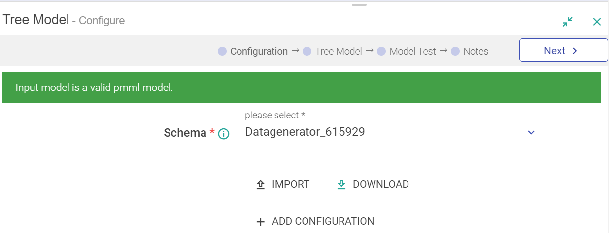
Field Description Schema Select the message from the drop-down list on which Analytics algorithm has to be applied. Import When the Model is Imported, two tabs are enabled – Import and Download. Download Downloads PMML file created either using Gathr UI or Import option. Add Configuration Configure additional parameters in Key – Value pair.
Input to this processor can only be provided as:
1. If you have a PMML file, representing Tree then you can directly import it. To do so you must choose Import Model as Yes and then click the Import button to load the file.
Once the model is imported, it is validated.
Tree Model tab is enabled and you can view Tree diagram of the model, as shown below.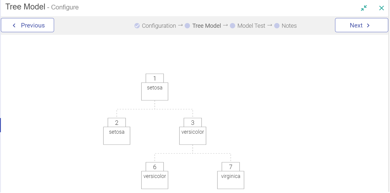
After the Tree Model view, you can then test the Model.
Test Model
You can test the model by clicking on Model Test tab.
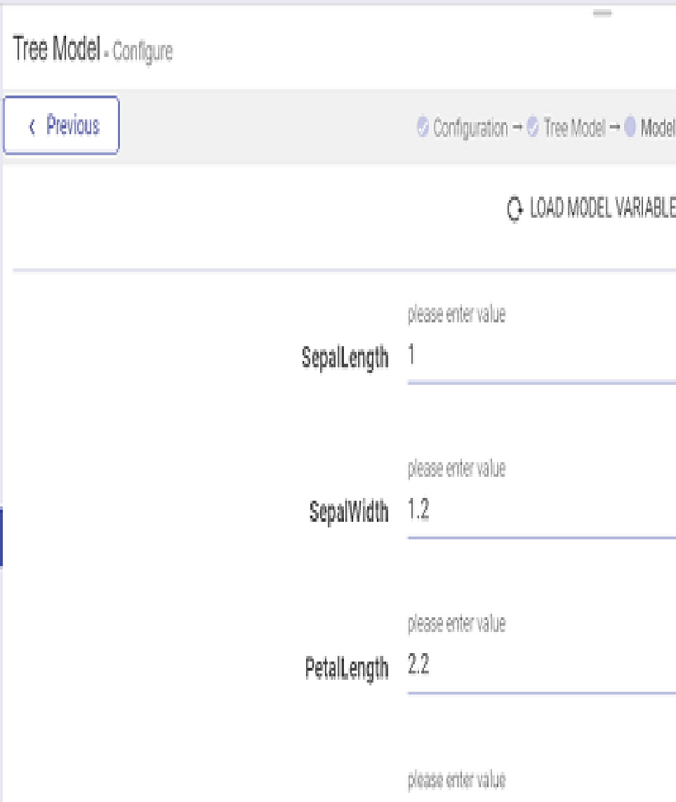
Specify value for all the model features and perform a single record test by clicking on TEST SINGLE RECORD button. The system will evaluate the model for this input and will show all the output parameters on screen.
Following is list of Algorithms of which PoJos created in H2O as models are supported for scoring over Gathr:
• Deep Learning
• Distributed Random Forest
• Gradient Boosting Machine
• K-Means
• Generalized Linear Modeling
• Naive Bayes
Scikit-learn provides a range of supervised and unsupervised learning algorithms via a consistent interface in Python.
The Algorithm types supported by Scikit are:
• Regression
• Classification
• Clustering
• Pipeline
To use a Scikit model for scoring, drag Scikit processor from analytics section on the pipeline canvas and right click on it for further configuration.
The configuration of SCIKIT is explained below:
Field | Description |
|---|---|
Algorithm | All predefined algorithms will be listed here.Select the algorithm on the basis of which prediction has to be done. |
Model Name | All the registered models of selected Algorithm will be listed here. Select the model which is to be used for prediction. |
For scoring using H2O model, drag H2O processor from analytics section on the pipeline canvas and right click on it for further configurations.
Configuring H2O Processor:
Field Description Algorithm All predefined algorithms will be listed here.Select the algorithm on the basis of which prediction has to be done. Model Name All the registered models of selected Algorithm will be listed here. Select the model which is to be used for prediction. Output Field Variable which holds the predicted output of model.
Models Page lists all the models which are trained through Gathr and models registered in Projects.
The Models home page consists of the list of models and brief of their configuration.
Property | Description |
Name | Name of the model. A mouseover on the name will display the Tags and Description configured with the model. |
Type | Type of model algorithm. e.g. Linear Regression, Logistic Regression, Decision Tree etc |
API | Underlying API of the model i.e. ML and H2O. |
Category | Model category i.e. Classification/ Regression/ Clustering. |
Active Version | Version of the model being used in the scoring pipeline. |
Pipeline Model | Indicates if the model is trained using ML Pipeline API. |
Actions | View model versions: Click to view the details of the model versions. Refer Model Version. Enable real time loading of the model: The check box enables every new successfully trained model version to be dynamically activated in the scoring pipeline. Latest version is the active version in the scoring pipeline. Delete: Allows you to delete the model along with version. |
On clicking the Model Version link, the model version details are displayed. 
Once you land on the model versions page, following are the properties displayed:
Property | Description |
Version | Version number of the model. The model version created will go in n+1 fashion and each model can have as many trained number of versions. |
Created On | Created date and time for the trained model. This field will be empty for a failed model. |
Rows (Train Set) | Number of data points in the trained dataset. |
Features | Count of features used to train the model. On hovering the field, Feature names will be shown. |
Metric | Evaluation metric selected by the user during model training. |
Value | Value of the selected metric. |
Status | Describes whether model is trained or failed. Possible values - Trained/Failed. |
Active | This selected model will be activated version of the model, which is used in the scoring pipeline. Activated version cannot be deleted. An activated version is check marked and Grey in color. If it is not, then there won’t be a check mark. (Refer above screenshot). To use the model-version in the scoring pipeline, click the check-mark. |
Actions | Open: Opens the model configuration, model details and performance visualization. Explained in Open Model Version. Download: Download the zipped file of the trained model version. Delete: Delete the selected model version. Enable Drift Detection: Enabling this feature will allow you to monitor the data drift patterns in the deployed model on regular intervals. Deploy as Service: To deploy (H2O MOJO, Scikit, Spark) models as REST endpoints on Gathr, select this option. |
Compare | Select a Metric to compare the model version. |

You can create different versions of the H2O MOJO model and use them in prediction pipelines.
To do so, enter the Models page, click on the View model versions (eye icon) under the Actions column. Here, you can view the existing versions of the model.
Click (+)Create Version button on the top of the screen.
The Create Version window pops up. Choose one of the model types:
• Distributed Random Forest
• Gradient Boosting Machine
• Generalized Linear Modeling
• Isolation Forest
There are two options to select the model source. These are:
• Upload local zip file
• Mention the HDFS connection and zip file location on the HDFS server
After mentioning the model source click Validate.
Once the model is successfully validated, click create for version creation.
Click on the link under the Active column to activate the model version. You can now use this version in the prediction pipeline.
To open a model’s version, you can click on the Open icon, under Actions, as shown below:
When you open the model version, depending on the Model Type-Regression or Classification (-Binary and Multi-class), the following properties are defined:
Classification | Regression |
|---|---|
Model Configuration | Model Configuration |
Model Details | Model Details |
Metrics | Metrics |
Confusion Metrics | Actual vs Predicted |
PR/ROC | Residuals |
Cumulative Gain | |
Decision Tree | |
Density Chart |
Not all Classification models will have all of the above mentioned properties but a few and same goes for Regression. Below explained is each property and the Model- Type under which it will be show.
Model Configuration lists the model configuration’s parameters (Key) and Values.
This tab is common for Classification and Regression models.
This tab enables you to visualize th Model. Depending on the type of models, below tabs are shown:
Pipeline Stages: The algorithm stages of the pipeline.
Intercept: The intercept is the expected mean value of Y when all x=0.
Coefficients: The coefficient for a feature represents the change in the mean response associated with a change in that feature, while the other features in the model are held constant. The sign of the coefficient indicates the direction of the relationship between the feature and the response.
Note: For Isotonic Regression, Naive Bayes, Model Details page shows only Pipeline Stages. Intercept and Coefficients are available for Linear and Logistic Regression Model.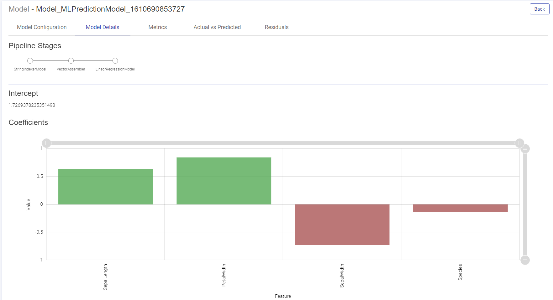
For Tree Based Models:
Feature Importance
This graph shows the estimation of importance of each feature used to train the model. Y-axis shows the feature names and X-axis shows the feature importance in percentage.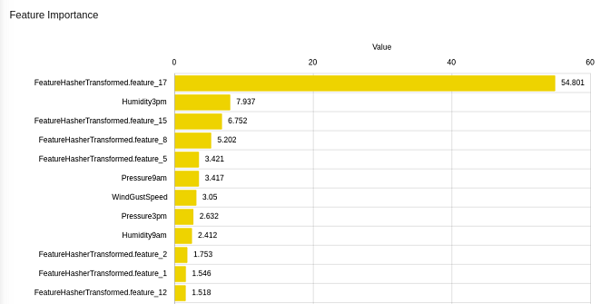
The metrics window will display all the performance indicators of the trained model.
For Isotonic Regression and Linear Regression Model, Evaluation Metrics are also generated, as shown below: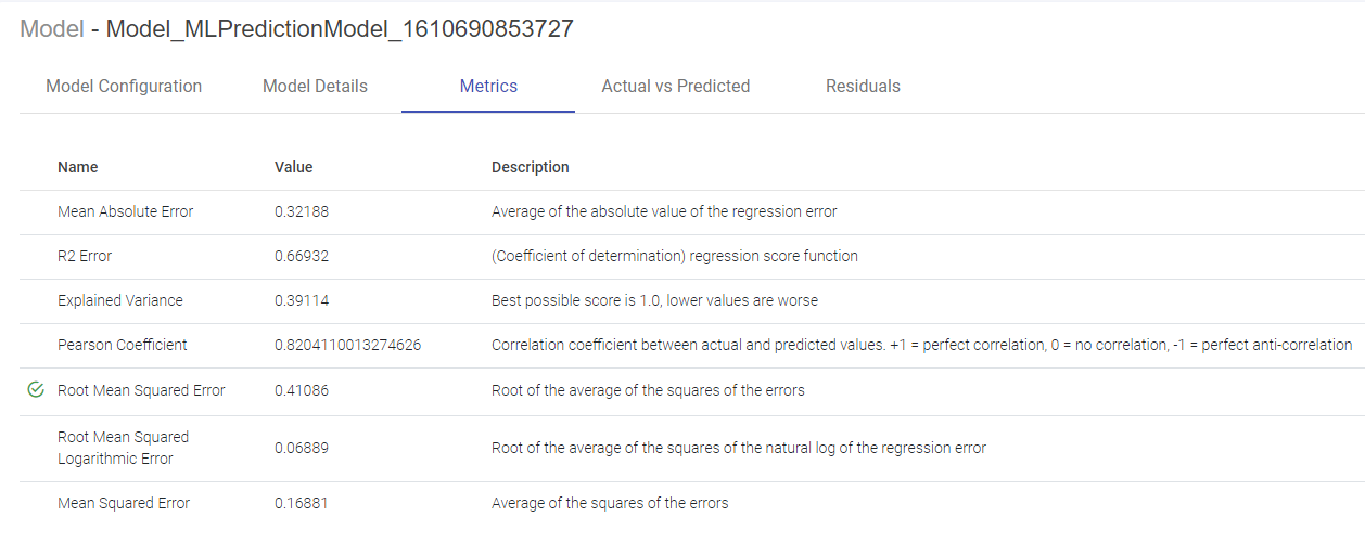
For Logistic Regression Model, Naive Bayes and Tree Based Models, performance indicators on which this classification model is evaluated such as Area under ROC, Area Under PR, Precision, Recall, Accuracy, FMeasure are generated, as shown below: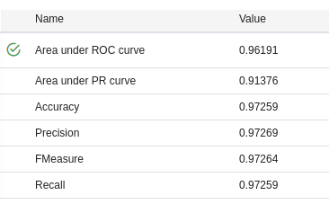
A confusion matrix is a table that is often used to describe the performance of a classification model (or “classifier”) on a set of test data for which the true values are known. Each row of the matrix represents the instances in an Actual class while each column represents the instances in an Predicted class.
Terms associated with Confusion matrix:
True Positives (TP): Number of instances where the model correctly predicts the positive class.
True Negatives (TN): Number of instances where the model correctly predicts the negative class.
False Positives (FP): Number of instances where the model incorrectly predicts the positive class.
False Negative (FN): Number of instances where model incorrectly predicts the negative class.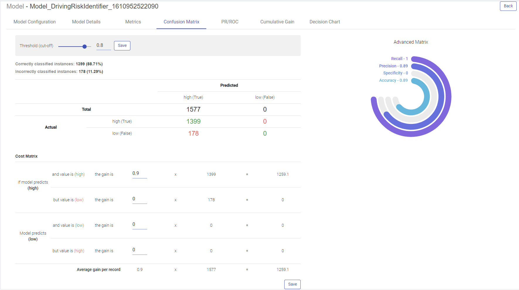
Advanced metrics
Recall, Precision, Specificity and Accuracy are calculated from the confusion matrix
Recall – TP/(TP + FN)
Precision – TP / (TP + FP)
Specificity – TN / (TN + FP)
Accuracy – TP + FN / (TP + FP + TN + FN)
ROC Curve:
ROC curves summarize the trade-off between the true positive rate and false positive rate for a predictive model using different probability thresholds.
X-axis shows false positive rate (False Positive/ (False Positive + True Negative)
Y-axis shows true positive rate (True Positive/ (True Positive + False Negative)
ROC curves are appropriate when the observations are balanced between each class.
Precision/Recall Curve:
Precision-Recall curves summarize the trade-off between the true positive rate (i.e. Recall) and the positive predictive value for a predictive model using different probability thresholds.
X-axis shows recall (True Positive/(True Positive + False Negative)
Y-axis shows precision (True Positive/(True Positive + False Positive)
Precision-recall curves are appropriate for imbalanced datasets.
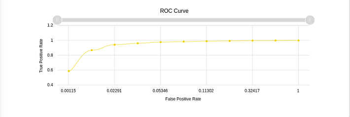
You can generate the Decision charts for binary classification models to understand a clear picture on the performance of the model.
The decision chart is a plot which is made by varying threshold and computing different values of the precision, recall and FMeasure scores.
Plots the probability vs probability density of different Classes. The minimum the overlapping area between the two curves, the better the model is.
Line Chart:
Two lines plotted on the graph i.e. one for the actual data and another one for the predicted data. This graph provides us information about how accurate model predictions are. All the predicted data points should overlap the predicted data points.
Scatter Plot:
This graph is plotted between the actual and predicted variables.
The regression line represents the linear line learned by the model.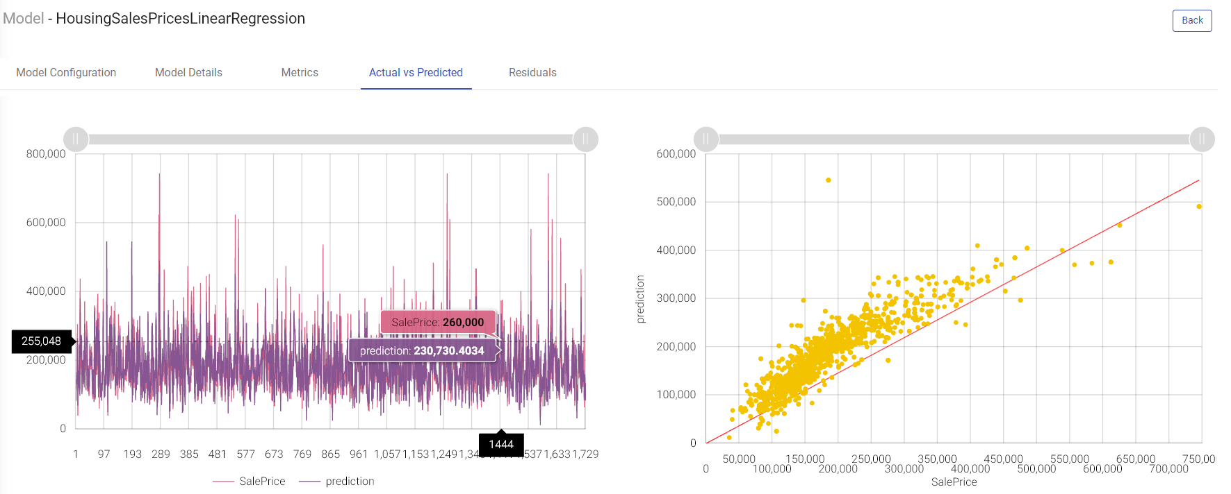
Cumulative Gain charts are used to evaluate performance of classification model. They measure how much better one can expect to do with the predictive model comparing without a model.
X-axis shows the estimated probability in descending order, splits into ten deciles.
Y-axis shows the percentage of cumulative positive responses in each decile i.e. cumulative positive cases captured in each decile divided by total number of positive cases.
Green dotted line denotes the random model.
Blue line is for the predictive model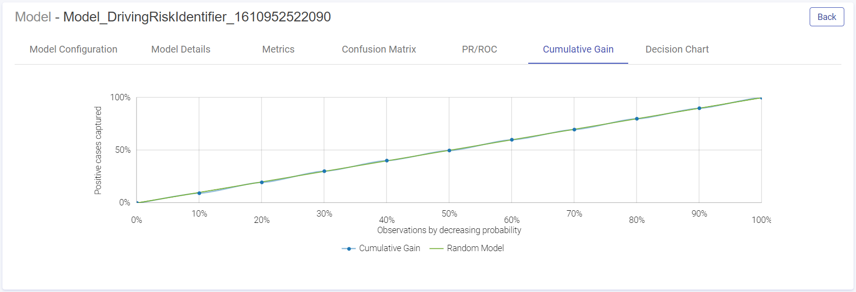
Residual error is the difference between the actual value and the predicted values for the output variable.
Shown below are the two plotted graphs to visualize the residuals error for the training model. In the first graph, a line chart is plotted between the residual error on the y axis and the count of the test data rows on the x axis. In the second plot, a histogram is made where the residuals are plotted on the x axis and the record count on the y axis. Histogram helps in providing intuition about how many records are having a particular range of residuals error: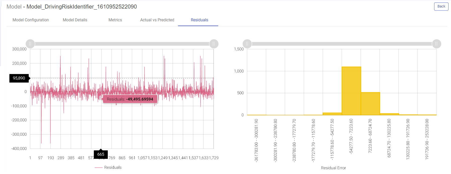
Model Deployment as Rest Service
Model as Service (H2O MOJO, Scikit, Spark)
We can now deploy (H2O MOJO, Scikit, Spark) models as REST endpoints on Gathr. In the models page, under the Actions column click on the eye icon to view model versions. You will be redirected to the models version page. Under the Actions column, click the Deploy as service option. Select the Local option. As you click Local, the window appears with fields of model name, version number and deployment port. Mention the port where the model will be deployed. Click Deploy.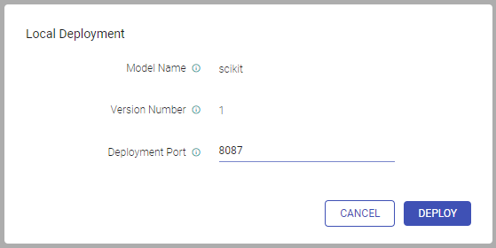
Once the model is successfully deployed, a message will be prompted on screen with the end point URL that can be copied on the clipboard.
The deployment indicator will also turn green specifying that the model has been locally deployed. As you hover over the button, you can see the end point URL of the locally deployed model.
Under the Actions column, the two new options that get visible are:
1.Terminate model service
2.Test model
Click the Test model. You may add headers in the test request.
In this window, an editable sample request is provided containing the features list for this model.
If you want to test a single record, mention the feature values in the request body or else you may upload a csv file to test multiple records.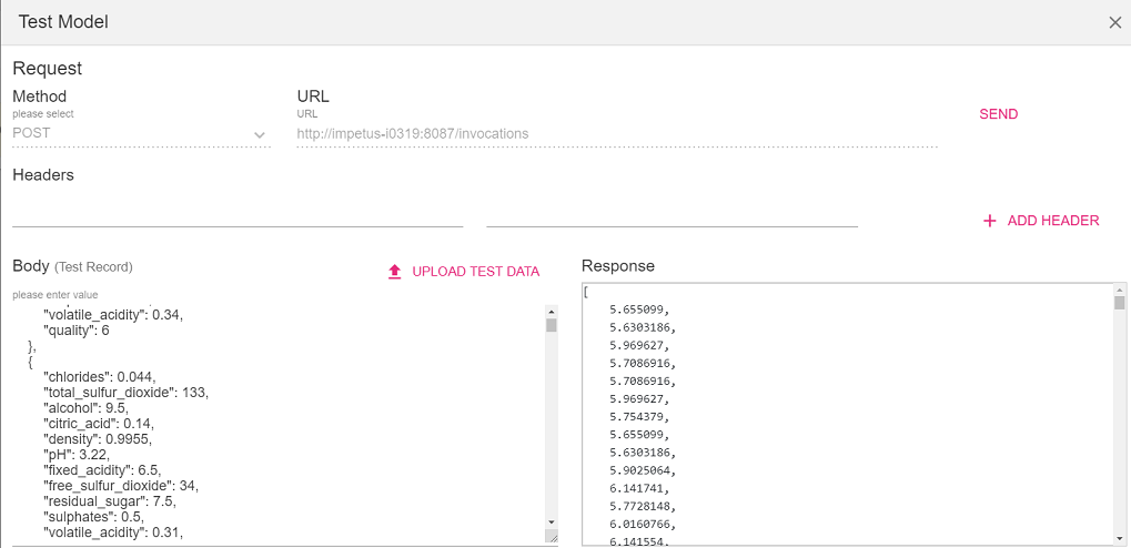
The uploaded file must contain the header row to map the feature values.
Click Send.
Terminate: You can terminate the model service deployed on the local server by clicking on the terminate button under the Actions column.
Note – To deploy H2O MOJO model as REST end point, make sure the H2O server is running. To start the embedded H2O server, please refer the installation guide.
After a model is deployed into production, the statistical properties of the data may change over time in unpredicted ways. Due to this, the predictions become less accurate. In Gathr, the user can monitor the data drift patterns in the deployed model on regular intervals.
Note: Data drift feature is supported only for the H2O models.
In the models page under actions column, click on the view model versions eye icon.
Under the Actions column, click on the Enable Drift Detection icon to configure drift detection. Upon clicking the icon, the Drift Detection configuration window pops up.
You may select the data source from which the model was trained from the below mentioned options:
1. Use Existing Dataset
2. Upload Sample Data
Note: If you are using the existing dataset its profile must be successfully run on the respective dataset. If you are uploading the sample data, the accuracy won’t be high as data drift would be calculated on the sample data.
Select the Dataset and choose its version if any. Click OK.
Note: To enable drift detection on a H2O model, make sure the H2O server is running. To start the embedded H2O server, please refer the installation guide.
To view the data drift for the last 7 days, click on View Data Drift icon under the Actions column.
In the data drift window, choose the pipeline for which you want to see the data drift. You can select the features for which you want to view the initial data stats, current data stats, Mean Drift% and IQR Drift%
The View Trends depicts the trend of data drift for the selected features: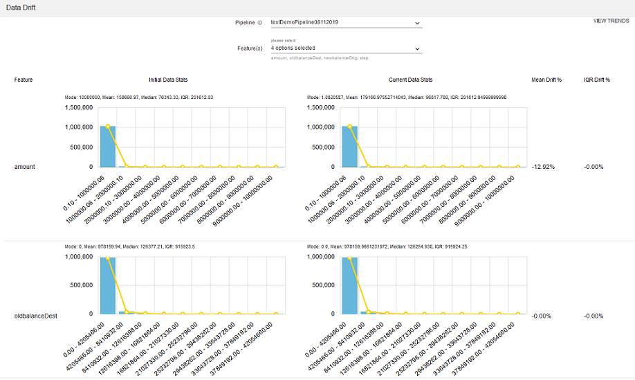
Data Drift Detector Configuration
To configure data drift with H20 (MOJO) model create a data pipeline with a source, H20 processor and data drift detector processor. Data drift detector processor is available under Analytics within the components palette of the data pipeline canvas.
Field Description Algorithm Select one of the algorithms: • Deep Learning • Distributed Random Forest • Gradient Boosting Machine • KMeans • Generalized Linear Modeling • Naïve Bayes Model Name Name of the model to be used for prediction. Threshold% for Mean Threshold% for mean drift notification in case of continuous column. Default value is 10. Threshold% for IQR Threshold% for IQR drift notification in case of continuous column. Default value is 10. Threshold Euclidean Distance Threshold Euclidean Distance for drift notification in case of categorical columns. Frequency Select the schedule for drift notification. Data Snapshot Window Window for data snapshot to calculate drift detection.
Note: The data drift feature for streaming use case will not be supported where Spark version is less than 2.4.